
PUBLIC
SAP HANA Platform 2.0 SPS 04
Document Version: 1.1 – 2019-10-31
SAP HANA Performance Guide for Developers
© 2019 SAP SE or an SAP aliate company. All rights reserved.
THE BEST RUN
Content
1 SAP HANA Performance Guide for Developers......................................6
2 Disclaimer................................................................. 7
3 Schema Design..............................................................8
3.1 Choosing the Appropriate Table Type...............................................8
3.2 Creating Indexes..............................................................9
Primary Key Indexes........................................................10
Secondary Indexes.........................................................11
Multi-Column Index Types....................................................12
Costs Associated with Indexes.................................................13
When to Create Indexes..................................................... 14
3.3 Partitioning Tables............................................................15
3.4 Query Processing Examples.....................................................16
3.5 Delta Tables and Main Tables....................................................18
3.6 Denormalization.............................................................19
3.7 Additional Recommendations....................................................21
4 Query Execution Engine Overview...............................................22
4.1 New Query Processing Engines.................................................. 24
4.2 ESX Example...............................................................25
4.3 Disabling the ESX and HEX Engines............................................... 26
5 SQL Query Performance......................................................28
5.1 SQL Process............................................................... 28
SQL Processing Components.................................................29
5.2 SAP HANA SQL Optimizer......................................................31
Rule-Based Optimization....................................................32
Cost-Based Optimization....................................................36
Decisions Not Subject to the SQL Optimizer.......................................48
Query Optimization Steps: Overview ............................................49
5.3 Analysis Tools.............................................................. 50
SQL Plan Cache...........................................................50
Explain Plan............................................................. 54
Plan Visualizer............................................................60
SQL Trace...............................................................68
SQL Optimization Step Debug Trace............................................70
SQL Optimization Time Debug Trace............................................77
2
P U B L I C
SAP HANA Performance Guide for Developers
Content
Views and Tables..........................................................82
5.4 Case Studies...............................................................83
Simple Examples..........................................................83
Performance Fluctuation of an SDA Query with UNION ALL............................95
Composite OOM due to Memory Consumed over 40 Gigabytes by a Single Query........... 103
Performance Degradation of a View after an Upgrade Caused by Calculation View Unfolding
..................................................................... 109
5.5 SQL Tuning Guidelines........................................................116
General Guidelines........................................................116
Avoiding Implicit Type Casting in Queries.........................................117
Avoiding Inecient Predicates in Joins ..........................................118
Avoiding Inecient Predicates in EXISTS/IN ......................................123
Avoiding Set Operations ....................................................124
Improving Performance for Multiple Column Joins..................................125
Using Hints to Alter a Query Plan..............................................126
Additional Recommendations................................................ 131
6 SQLScript Performance Guidelines.............................................134
6.1 Calling Procedures.......................................................... 134
Passing Named Parameters................................................. 135
Changing the Container Signature.............................................136
Accessing and Assigning Variable Values........................................ 136
Assigning Scalar Variables...................................................138
6.2 Working with Tables and Table Variables........................................... 138
Checking Whether a Table or Table Variable is Empty................................138
Determining the Size of a Table Variable or Table...................................140
Accessing a Specic Table Cell................................................141
Searching for Key-Value Pairs in Table Variables....................................142
Avoiding the No Data Found Exception..........................................144
Inserting Table Variables into Other Table Variables .................................144
Inserting Records into Table Variables.......................................... 145
Updating Individual Records in Table Variables.................................... 147
Deleting Individual Records in Table Variables.....................................148
6.3 Blocking Statement Inlining with the NO_INLINE Hint..................................150
6.4 Skipping Expensive Queries.................................................... 151
6.5 Using Dynamic SQL with SQLScript.............................................. 152
Using Input and Output Parameters............................................153
6.6 Simplifying Application Coding with Parallel Operators.................................154
Map Merge Operator...................................................... 154
Map Reduce Operator......................................................156
6.7 Replacing Row-Based Calculations with Set-Based Calculations.......................... 162
6.8 Avoiding Busy Waiting........................................................165
SAP HANA Performance Guide for Developers
Content
P U B L I C 3
6.9 Best Practices for Using SQLScript...............................................166
Reduce the Complexity of SQL Statements ...................................... 167
Identify Common Sub-Expressions............................................ 167
Multi-Level Aggregation.....................................................167
Reduce Dependencies..................................................... 168
Avoid Using Cursors.......................................................168
Avoid Using Dynamic SQL...................................................170
7 Optimization Features in Calculation Views.......................................171
7.1 Calculation View Instantiation...................................................172
7.2 Setting Join Cardinality....................................................... 176
Join Cardinality.......................................................... 177
Examples...............................................................178
7.3 Optimizing Join Columns......................................................198
Optimize Join Columns Option............................................... 198
Prerequisites for Pruning Join Columns......................................... 199
Example...............................................................201
7.4 Using Dynamic Joins.........................................................210
Dynamic Join Example..................................................... 211
Workaround for Queries Without Requested Join Attributes...........................217
7.5 Union Node Pruning.........................................................220
Pruning Conguration Table.................................................222
Example with a Pruning Conguration Table......................................222
Example with a Constant Mapping.............................................225
Example Tables..........................................................227
7.6 Inuencing the Degree of Parallelization...........................................228
Example: Create the Table.................................................. 229
Example: Create the Model..................................................230
Example: Apply Parallelization Based on Table Partitions.............................233
Example: Apply Parallelization Based on Distinct Entries in a Column....................236
Verifying the Degree of Parallelization.......................................... 238
Constraints.............................................................241
7.7 Using "Execute in SQL Engine" in Calculation Views...................................242
Impact of the "Execute in SQL Engine" Option ....................................243
Checking Whether a Query is Unfolded......................................... 246
Inuencing Whether a Query is Unfolded........................................246
7.8 Push Down Filters in Rank Nodes................................................248
7.9 Condensed Performance Suggestions............................................ 248
7.10 Avoid Long Build Times for Calculation Views....................................... 250
Check Whether Long Build Times are Caused by Technical Hierarchies...................250
Avoid Creating Technical Hierarchies (Optional)................................... 251
4
P U B L I C
SAP HANA Performance Guide for Developers
Content
1 SAP HANA Performance Guide for
Developers
The SAP HANA Performance Guide for Developers provides an overview of the key features and characteristics
of the SAP HANA platform from a performance perspective. While many of the optimization concepts and
design principles that are common for almost all relational database systems also apply to SAP HANA, there
are some SAP HANA-specic aspects that are highlighted in this guide.
The guide starts with a discussion of physical schema design, which includes the optimal choice between a
columnar and row store table format, index creation, as well as further aspects such as horizontal table
partitioning, denormalization, and others.
After a brief overview of the query processing engines used in SAP HANA, the next section of the guide focuses
on SQL query performance and the techniques that can be applied to improve execution time. It also describes
how the analysis tools can be used to investigate performance issues and illustrates some key points through a
selection of cases studies. It concludes by giving some specic advice about writing and tuning SQL queries,
including general considerations such as programming in a database-friendly and more specically column
store-friendly way.
The focus of the nal sections of the guide is on the SQLScript language provided by SAP HANA for stored
procedure development, as well as the calculation engine, which provides more advanced features than those
available through the SQL query language. These sections discuss recommended programming patterns that
yield optimal performance as well as anti-patterns that should be avoided.
Related Information
SAP HANA SQL and System Views Reference
SAP HANA SQLScript Reference
SAP HANA Modeling Guide for XS Advanced Model
6
P U B L I C
SAP HANA Performance Guide for Developers
SAP HANA Performance Guide for Developers

2 Disclaimer
This guide presents generalized performance guidelines and best practices, derived from the results of internal
testing under varying conditions. Because performance is aected by many factors, it cannot be guaranteed
that these guidelines will improve performance in each case. We recommend that you regard these guidelines
as a starting point only.
As an example, consider the following. You have a data model that consists of a star schema. The general
recommendation would be to model it using a calculation view because this allows the SAP HANA database to
exploit the star schema when computing joins, which could improve performance. However, there might also
be reasons why this would not be advisable. For example:
● The number of rows in some of the dimension tables is much bigger than you would normally expect, or
the fact table is much smaller.
● The data distribution in some of the join columns appears to be heavily skewed in ways you would not
expect.
● There are more complex join conditions between the dimension and fact tables than you would expect.
● A query against such tables does not necessarily always involve all tables in the star schema. It could be
that only a subset of those tables is touched by the query, or it could also be joined with other tables
outside the star schema.
Performance tuning is essentially always a trade-o between dierent aspects, for example, CPU versus
memory, or maintainability, or developer eectiveness. It therefore cannot be said that one approach is always
better.
Note also that tuning optimizations in many cases create a maintenance problem going forward. What you may
need to do today to get better performance may not be valid in a few years' time when further optimizations
have been made inside the SAP HANA database. In fact, those tuning optimizations might even prevent you
from beneting from the full SAP HANA performance. In other words, you need to monitor whether specic
optimizations are still paying o. This can involve a huge amount of eort, which is one of the reasons why
performance optimization is very expensive.
Note
In general, the SAP HANA default settings should be sucient in almost any application scenario. Any
modications to the predened system parameters should only be done after receiving explicit instruction
from SAP Support.
SAP HANA Performance Guide for Developers
Disclaimer
P U B L I C 7
3 Schema Design
The performance of query processing in the SAP HANA database depends heavily on the way in which the data
is physically stored inside the database engine.
There are several key characteristics that inuence the query runtime, including the choice of the table type
(row or column storage), the availability of indexes, as well as (horizontal) data partitioning, and the internal
data layout (delta or main). The sections below explain how these choices complement each other, and also
which combinations are most benecial. The techniques described can also be used to selectively tune the
database for a particular workload, or to investigate the behavior and inuencing factors when diagnosing the
runtime of a given query. You might also want to evaluate the option of denormalization (see the dedicated
topic on this subject), or consider making slight modications to the data stored by your application.
Related Information
Choosing the Appropriate Table Type [page 8]
Creating Indexes [page 9]
Partitioning Tables [page 15]
Delta Tables and Main Tables [page 18]
Query Processing Examples [page 16]
Denormalization [page 19]
3.1 Choosing the Appropriate Table Type
The default table type of the SAP HANA database system is columnar storage.
Columnar storage is particularly benecial for analytical (OLAP) workloads, since it provides superior
aggregation and scan performance on individual attributes, as well as highly sophisticated data compression
capabilities that allow the main memory footprint of a table to be signicantly reduced. At the same time, the
SAP HANA column store is also capable of sustaining high throughput and good response times for
transactional (OLTP) workloads. As a result, columnar storage should be the preferred choice for most
scenarios.
However, there are some cases where row-oriented data storage might give a performance advantage. In
particular, it might be benecial to choose the row table type when the following apply:
● The table consists of a very small data set (up to a few thousand records), so that the lack of data
compression in the row store can be tolerated.
● The table is subject to a high-volume transactional update workload, for example, performing frequent
updates on a limited set of records.
● The table is accessed in a way where the entire record is selected (select *), it is accessed based on a
highly selective criterion (for example, a key or surrogate key), and it is accessed extremely frequently.
8
P U B L I C
SAP HANA Performance Guide for Developers
Schema Design

If a table does not full at least one of the criteria given above, it should not be considered for row-based
storage. In general, row-based storage should be considered primarily for extreme OLTP scenarios requiring
query response times within the microsecond range.
Also note that cross-engine joins that include row and column store tables cannot be handled with the same
eciency as in row-to-row and column-to-column joins. This should also be taken into account when
considering whether to change the storage type, as join performance can be signicantly aected.
A large row store consisting of a large number of row store tables or several very large row store tables also has
a negative impact on the database restart time, because currently the whole row store is loaded during a
restart. An optimization has been implemented for a planned stop and start of the database, but in the event of
a crash or machine failure that optimization does not work.
The main criteria for column-based storage and row-based storage are summarized below:
Column Store
Row Store
Tables with many rows (more than a couple of 100,000), be
cause of better compression in the column store
Very large OLTP load on the table (high rate of single up
dates, inserts, or deletes)
Note that select * and select single are not sucient criteria
for putting a table into row-based storage.
Tables with a full-text index
Tables used in an analytical context and containing business-
relevant data
Note
If neither ROW nor COLUMN is specied in the CREATE TABLE statement, the table that is created is a
column table. However, because this was not the default behavior in SAP HANA 2.0 SPS 02 and earlier, it is
generally recommended to always use either the COLUMN or ROW keyword to ensure that your code works
for all versions of SAP HANA.
3.2 Creating Indexes
The availability of index structures can have a signicant impact on the processing time of a particular table,
both for column-based and row-based data storage.
For example, when doing a primary-key lookup operation (where exactly one or no record is returned), the
availability of an index may reduce the query processing time from a complete table scan (in the worst case)
over all n records of a table, to a logarithmic processing time in the number of distinct values k (log k). This
could easily reduce query runtimes from several seconds to a few milliseconds for large tables.
The sections below discuss the dierent access paths and index options for the column store. The focus is on
the column store because columnar storage is used by default and is the preferred option for most scenarios.
However, similar design decisions exist for row-store tables.
Related Information
Primary Key Indexes [page 10]
SAP HANA Performance Guide for Developers
Schema Design
P U B L I C 9
Secondary Indexes [page 11]
Multi-Column Index Types [page 12]
Costs Associated with Indexes [page 13]
When to Create Indexes [page 14]
3.2.1 Primary Key Indexes
Most tables in the SAP environment have a primary key, providing a unique identier for each individual row in
a table. The key typically consists of several attributes. The SAP HANA column store automatically creates
several indexes for each primary key.
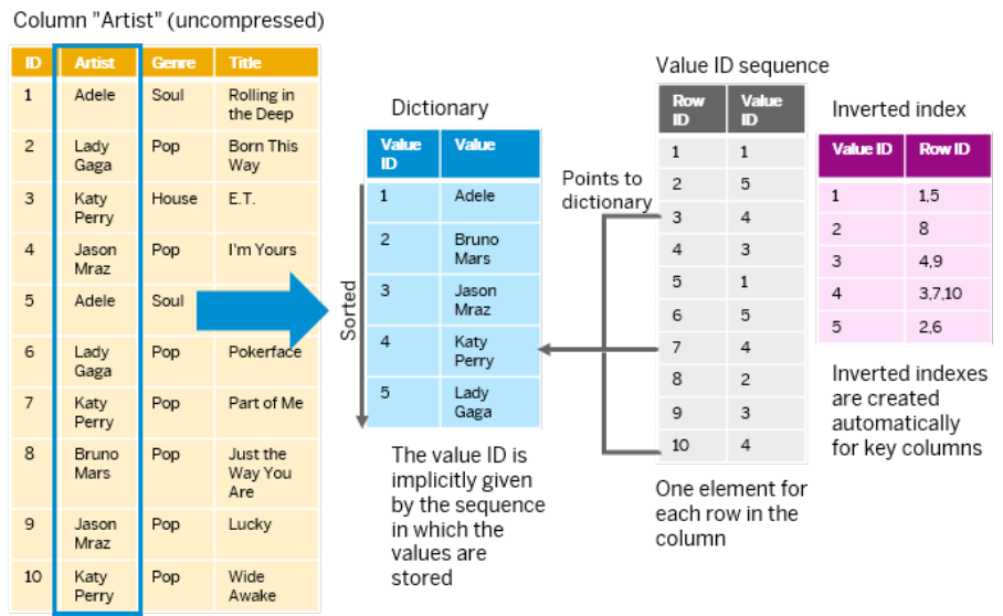
For each individual key attribute of a primary key, an implicit single-column index (inverted index) is created as
an extension to the corresponding column. Inverted indexes are light-weight data structures that map column
dictionary value IDs to the corresponding row IDs. The actual data in the column is stored as an array of value
IDs, also called an index vector.
The example below illustrates the direct mapping of dictionary values IDs to table row IDs using an inverted
index (shown on the right). The column dictionary contains all existing column values in sorted order, but it
does not provide any information about which rows of the table contain the individual values. The mapping
between the dictionary value IDs and the related table row IDs is only available through the inverted index.
Without the index, the whole column would have to be scanned to nd a specic value:
If more than one attribute is part of the key, a concatenated index is also created for all the involved attributes.
The concatenated column values (index type INVERTED VALUE) or the hash values of the indexed columns
(index type INVERTED HASH) are stored in an internal index key column (also called a concat attribute), which
is added to the table. Note that this does not apply to the index type INVERTED INDIVIDUAL.
10
P U B L I C
SAP HANA Performance Guide for Developers
Schema Design
For example:
● A table with a primary key on (MANDT, KNR, RNR) will have separate inverted indexes on the column
MANDT, on the column KNR, and on the column RNR.
Depending on the index type, the primary key will also have a resulting concatenated index for the three
attributes.
● A table with a surrogate primary key SUR (that is, an articial identier such as a GUID or monotonically
increasing counter) will have only one individual index on the attribute SUR. It will not have a concatenated
index, since there is only one key attribute.
Related Information
Multi-Column Index Types [page 12]
3.2.2 Secondary Indexes
Apart from a primary key, which provides a unique identier for each row and is supported by one or multiple
corresponding indexes as outlined above, an arbitrary number of secondary indexes can be created. Both
unique and non-unique secondary indexes are supported.
Internally, secondary indexes translate into two dierent variants, depending on the number of columns that
are involved:
● Indexes on individual columns
When creating an index on an individual column, the column store creates an inverted list (inverted index)
that maps the dictionary value IDs to the corresponding entries in the index vector. Internally, two index
structures are created, one for the delta table and one for the main table.
When this index is created for the row store, only one individual B+ tree index is created.
● Indexes on multiple columns (concatenated indexes)
A multi-column index can be helpful if a specic combination of attributes is queried frequently, or to
speed up join processing where multiple attributes are involved. Note that when a concatenated index is
created, no individual indexes are created for the constituent attributes (this is only done for the primary
key, where individual indexes are also created for each of these attributes).
The column store supports the inverted value index, inverted hash index, and inverted individual index for
multi-column indexes.
When a concatenated index is created for the row store, only one individual B tree index is created.
Related Information
Multi-Column Index Types [page 12]
CREATE INDEX Statement (Data Denition)
SAP HANA Performance Guide for Developers
Schema Design
P U B L I C 11
3.2.3 Multi-Column Index Types
The column store supports the inverted value index, inverted hash index, and inverted individual index for
multi-column indexes. The inverted value index is the default index type for multi-column keys.
Inverted Value Indexes
An inverted value index consists of the concatenation string of all values of the attributes for each individual
row. Internally, an inverted value index consists of three major components: A dictionary that contains the
concatenation of all attribute values, an index vector, and an inverted list (inverted index) that maps the
dictionary value IDs to the corresponding records.
For each composite key or index, a new internal index key column (also called a concat attribute) is added to
the table. This column, which is typically hidden and persisted, is handled like any other database column.
In addition, for each primary key and constituent of the primary key, a separate inverted index is created
automatically. Note that this does not occur for secondary keys.
Concatenated indexes should be used with care because their main memory footprint tends to be signicant,
given the fact that an additional dictionary needs to be created.
Inverted Hash Indexes
If an index consists of many columns with long values, storing the concatenated keys can lead to signicant
memory consumption. The inverted hash index helps reduce memory consumption and generally results in a
signicantly smaller memory footprint (30% or more). For indexes of this type, the dictionary of the internal
index key column stores hash values of the indexed columns.
Inverted hash indexes can be used for primary indexes and unique indexes that consist of at least two columns.
They are not recommended for non-unique secondary indexes because they can cause performance issues.
Note that the memory footprint after a join is always at least the same as that for inverted value indexes.
Inverted Individual Indexes
Unlike an inverted value index or inverted hash index, an inverted individual index does not require a dedicated
internal index key column because a light-weight inverted index structure is created instead for each individual
index column. Due to the absence of this column, the memory footprint can be signicantly reduced.
Inverted individual indexes can be used for multi-column primary indexes and unique indexes. Good candidates
for inverted individual indexes are those where all the following conditions are met:
● They are large multi-column indexes that are required for uniqueness or primary key purposes.
● There is a selective index column that is typically used in a WHERE clause. Based on column statistics, this
column will be processed rst during a uniqueness check and query processing to obtain a small candidate
12
P U B L I C
SAP HANA Performance Guide for Developers
Schema Design
result set. In the absence of a selective column, more column values need to be compared, resulting in a
larger query processing overhead.
● They are not accessed frequently during query processing of a critical workload (unless a slight
performance overhead is acceptable).
Bulk-loading scenarios can benet from the inverted individual index type because the delta merge of the
internal index key columns in not needed and I/O is reduced. However, queries that could use a concatenated
index, such as primary key selects, will be up to 20% slower with inverted individual indexes compared to
inverted value indexes. For special cases like large in-list queries, the impact may be even higher. Join queries
could also have an overhead of about 10%.
For DML insert, update, and delete operations, there are performance gains because less data is written to the
delta and redo log. However, depending on the characteristics of the DML change operations, the uniqueness
check and WHERE clause processing may be more complex and therefore slower.
Note that the inverted individual index type is not needed for non-unique multi-column indexes because
inverted indexes can simply be created on the individual columns. This will result in the same internal index
structures.
Related Information
CREATE INDEX Statement (Data Denition)
3.2.4 Costs Associated with Indexes
Indexes entail certain costs. Memory consumption and incremental maintenance are two major cost factors
that need to be considered.
Memory Consumption
To store the mapping information of value IDs to records, each index uses an inverted list that needs to be kept
in main memory. This list typically requires an amount of memory that is of the same order of magnitude as the
index vector of the corresponding attribute. When creating a concatenated index (for more information, see
above), there is even more overhead because an additional dictionary containing the concatenated values of all
participating columns needs to be created as well. It is dicult to estimate the corresponding overhead, but it
is usually notably higher than the summed-up size of the dictionaries of the participating columns. Therefore,
concatenated indexes should be created with care.
The memory needed for inverted individual indexes includes the memory for inverted indexes on all indexed
columns. This memory usage can be queried as a sum of M_CS_COLUMNS.MEMORY_SIZE_INDEX for all
indexed columns.
The main advantage of the inverted individual index is its low memory footprint. The memory needed for
inverted individual indexes is much smaller than the memory used for the internal index key column that is
required for inverted value and inverted hash indexes. In addition, the data and log I/O overhead, table load
SAP HANA Performance Guide for Developers
Schema Design
P U B L I C 13

time, CPU needed for the delta merge, and the overhead of DML update operations are also reduced because
an internal column does not need to be maintained. Similarly, the DDL to create an inverted individual index is
also much faster than for the other index types because the concatenated string does not need to be
generated.
Incremental Maintenance
Whenever a DML operation is performed on the base table, the corresponding index structures need to be
updated as well (for example, by inserting or deleting entries). These additional maintenance costs add to the
costs on the base relation, and, depending on the number of indexes created, the number of attributes in the
base table, and the number of attributes in the individual indexes, might even dominate the actual update time.
Again, this requires that care is taken when creating additional indexes.
3.2.5 When to Create Indexes
Indexes are particularly useful when a query contains highly selective predicates that help to reduce the
intermediate results quickly.
The classic example for this is a primary key-based select that returns a single row or no row. With an index,
this query can be answered in logarithmic time, while without an index, the entire table needs to be scanned in
the worst case to nd the single row that matches the attribute, that is, in linear time.
However, besides the overhead for memory consumption and the maintenance costs associated with indexes,
some queries do not really benet from them. For example, an unselective predicate such as the client
(German: Mandant) does not lter the dataset much in most systems, since they typically have a very limited
set of clients and one client contains virtually all the entries. On the other hand, in cases of data skew, it could
be benecial to have an index on such a column, for example, when frequently searching for MANDT='000' in a
system that has most data in MANDT='200'.
Consider the following recommendations when manually creating indexes:
Recommendation
Details
Avoid non-unique indexes Columns in a column table are inherently index-like and there
fore do not usually benet from additional indexes. In some sce
narios (for example, multiple-column joins or unique con
straints), indexes can further improve performance.
Start without any indexes and then add them if needed.
Create as few indexes as possible
Every index imposes an overhead in terms of space and per
formance, so you should create as few indexes as possible.
Ensure that the indexes are as small as possible Specify as few columns as possible in an index so that the
space overhead is minimized.
14 P U B L I C
SAP HANA Performance Guide for Developers
Schema Design

Recommendation Details
Prefer single-column indexes in the column store Single-column indexes in the column store have a much lower
space overhead because they are just light-weight data struc
tures created on top of the column structure. Therefore, you
should use single-column indexes whenever possible.
Due to the in-memory approach in SAP HANA environments, it
is generally sucient to dene an index on only the most selec
tive column. (In other relational databases, optimal perform
ance can often only be achieved by using a multi-column index.)
For information about when to combine indexes with partitioning, see Query Processing Examples.
Related Information
Query Processing Examples [page 16]
3.3 Partitioning Tables
For column tables, partitioning can be used to horizontally divide a table into dierent, physical parts that can
be distributed to the dierent nodes in a distributed SAP HANA database landscape.
Partitioning criteria include range, hash, and round-robin partitioning. From a query processing point of view,
partitioning can be used to restrict the amount of data that needs to be analyzed by ruling out irrelevant parts
in a rst step (partition pruning). For example, let's assume a table is partitioned based on a range predicate
operating on a YEAR attribute. When a query with a predicate on YEAR now needs to be processed (for
example, select count(1) from table where year=2013), the system can restrict the aggregation to
the rows in the individual partition for year 2013 only, instead of taking all available partitions into account.
While partition pruning can dramatically improve processing times, it can only be applied if the query
predicates match the partitioning criteria. For example, partitioning a table by YEAR as above is not
advantageous if the query does not use YEAR as a predicate, for example, select count(1) from table
where MONTH=4. In the latter case, partitioning may even be harmful, since several physical storage
containers need to be accessed to answer the query, instead of just a single one as in the unpartitioned case.
Therefore, to use partitioning to speed up query processing, the partitioning criteria need to be chosen in a way
that supports the most frequent and expensive queries that are processed by the system. For information
about when to combine partitioning with indexes, see Query Processing Examples.
Costs of Partitioning
Internally, the SAP HANA database treats partitions as physical data containers, similar to tables. In particular,
this means that each partition has its own private delta and main table parts, as well as dictionaries that are
SAP HANA Performance Guide for Developers
Schema Design
P U B L I C 15

separate from those of the other partitions. As a result and depending on the actual value distribution and
partitioning criteria, the main memory consumption of a table might increase or decrease when it is changed
from a non-partitioned to a partitioned table. While this does not initially appear very intuitive, the root cause
for this lies in the dictionary compression that is applied.
For example:
● Increased memory consumption due to partitioning
A table has two attributes, MONTH and YEAR, and contains data for all 12 months and two distinct years
(2013 and 2014). When the table is partitioned by YEAR, the dictionary for the MONTH attribute needs to be
held in memory twice (both for 2013 and 2014), therefore increasing memory consumption.
● Decreased memory consumption due to partitioning
A table has two attributes, GENDER and FIRSTNAME, and stores data about German customers. When the
table is partitioned by GENDER, it is divided into two groups (female and male). In Germany, there is a
limited set of rst names for both females and males. As a result, the FIRSTNAME dictionaries are implicitly
partitioned as well into two almost distinct groups, both containing almost n/2 distinct values, compared
to the unpartitioned table with n distinct values. Therefore, to represent those values in the index vector,
only n-1 bits are required instead of n bits in the original table. As there is virtually no redundancy in the
dictionaries, memory consumption can be reduced by partitioning.
3.4 Query Processing Examples
The examples below show how the dierent access paths and optimization techniques described above can
signicantly inuence query processing .
Exploiting Indexes
This example shows how a query with multiple predicates can potentially benet from the dierent indexes that
are available. The query used in the example is shown below, where the table FOO has a primary key for MANDT,
BELNR, and POSNR:
SELECT * FROM FOO
WHERE MANDT='999' and BELNR='xx2342'
No Indexes: Attribute Scans
A straightforward plan would be to scan both the attributes MANDT and BELNR to nd all matching rows, and
then materialize the result set for those rows where both criteria have been fullled. Since the column store
uses dictionary compression, the system rst needs to look up the corresponding value IDs from the dictionary
during predicate evaluation (MANDT='999' and BELNR='xx2342'). It does this with a binary search operation
on the sorted dictionary for the main table, which means
log k, where k is the number of distinct values in the
main table. For the delta table, there are auxiliary structures that allow the value IDs to be retrieved with the
same degree of complexity from the unsorted delta dictionary. After that, the scan operation can be performed
to compare the value IDs. The scan operations are run sequentially so that if the rst scan already reduces the
result set signicantly, further scanning can be avoided and the values of the individual rows looked up instead.
16
P U B L I C
SAP HANA Performance Guide for Developers
Schema Design
This is also one of the reasons why query execution tries to start with the evaluation of the most selective
predicate rst (for example, it is more likely that BELNR will be evaluated before MANDT, depending on the
selectivity estimations).
Conceptually, the runtime for these scans is 2*n, where n is the number of values in the table. However, the
actual runtime depends on the number of distinct values in the corresponding column. For attributes with very
few distinct values (for example,
MANDT), it might be sucient to use a small number of bits to encode the
dictionary values (for example, 2 bits). Since the SAP HANA database scan operators use SIMD instructions
during processing, multiple-value comparisons can be done at the same time, depending on the number of bits
required for representing an entry. Therefore, a scan of n records with 2 bits per value is notably faster than a
scan of n records with 6 bits (an almost linear speedup).
In the last step of query processing, the result set needs to be materialized. Therefore, for each cell (that is,
each attribute in each row), the actual value needs to be retrieved from the dictionary in constant time.
Single-Column Indexes
To improve the query processing time, the system can use the single-column indexes that are created for each
column of the key. Instead of doing the column scan operations for MANDT and BELNR, the indexes can be used
to retrieve all matching records for the given predicates, reducing the evaluation costs from a scan to a
constant-time lookup operation for the column store. The other costs (combining the two result sets,
dictionary lookup, and result materialization) remain the same.
Concatenated Indexes
When a concatenated index is available, it is preferrable to use it for query processing. Instead of having to do
two individual index-backed search operations on MANDT and BELNR and combine the results afterwards (AND),
the query can be answered by a single index-access operation if a concatenated index on (MANDT, BELNR) is
available. In this particular example, this is not the case, because the primary key also contains the POSNR
predicate and therefore cannot be used directly. However, in this special case, the concatenated index of the
primary key can still be exploited. Since the query uses predicates that form a prex of the primary key, the
search can be regarded internally as semantically equivalent to SELECT * FROM FOO WHERE MANDT='999'
and BELNR='xx2342' and POSNR like '%'. Since the SAP HANA database engine internally applies a
similar rewrite (with a wildcard as the sux of the concatenated attributes), the concatenated index can still be
used to accelerate the query.
When this example is actually executed in the system, the concatenated index is exploited as described above.
Indexes Versus Partitioning
Both indexes and partitioning can be used to accelerate query processing by avoiding expensive scans. While
partitioning and partition pruning reduce the amount of data to be scanned, the creation of indexes provides
additional, alternate access paths at the cost of higher memory consumption and maintenance.
Partitioning
If partition pruning can be applied, this can have the following benets:
● Scan operations can be limited to a subset of the data, thereby reducing the costs of the scan.
● Partitioning a table into smaller chunks might enable the system to represent large query results in a more
ecient manner. For example, a result set of hundreds of thousands of records might not be represented
SAP HANA Performance Guide for Developers
Schema Design
P U B L I C 17
as a bit vector for a huge table with billions of records, but this might be feasible if the table were
partitioned into smaller chunks. Consequently, result set comparisons (AND/OR of several predicates) and
handling might be more ecient in the partitioned case.
Note that these benets heavily depend on having matching query predicates. For example, partitioning a table
by YEAR is not benecial for a query that does not include YEAR as a predicate. In this case, query processing
will actually be more expensive.
Indexes
Indexes can speed up predicate evaluation. The more selective a predicate is, the higher the gain.
Combining Partitioning and Indexes
For partitioning, the greatest potential for improvement is when the column is not very selective. For indexing, it
is when the column is selective. Combining these techniques on dierent columns can be very powerful.
However, it is not benecial to use them on the same column for the sole purpose of speeding up query
processing.
3.5 Delta Tables and Main Tables
Each column store table consists of two distinct parts, the main table and the delta table. While the main table
is read only, heavily compressed, and read optimized, the delta table is responsible for reecting changes made
by DML operations such as INSERT, UPDATE, and DELETE. Depending on a cost-based decision, the system
automatically merges the changes of the delta table into the main table (also known as delta merge) to improve
query processing times and reduce memory consumption, since the main table is much more compact.
The existence and size of the delta table might have a signicant impact on query processing times:
● When the delta table is not empty, the system needs to evaluate the predicates of a query on both the delta
and main tables, and combine the results logically afterwards.
● When a delta table is quite large, query processing times may be negatively aected, since the delta table
is not as read optimized as the main table.
Therefore, by merging the delta table into the main table to reduce main memory consumption, delta merges
might also have a positive impact on reducing query processing times. However, a delta merge also has an
associated cost, which is mostly linear to the size of the main table. A delta merge should therefore only be
performed after weighing the improvement in memory consumption and query processing times against this
cost. In the case of automatic merges, it has already been considered in the cost function.
Data Compression
After merging the contents of the delta table into the main table during the delta merge process, the system
might optionally run an additional data compression step to reduce the main memory footprint of the main
table part. This process is also known as optimize compression. Internally, the SAP HANA database system
contains multiple compression methods (run length encoding, sparse coding, default value, and so on). While
the most ecient compression mechanisms are automatically chosen by the system, the compression
mechanism that is applied might also aect the query processing times. It is normally not necessary to
18
P U B L I C
SAP HANA Performance Guide for Developers
Schema Design
manually alter the compression methods, or even uncompress the table, but this can be done when there is a
problem with data compression. Generally, however, you should contact SAP Support when there is a problem
with data compression.
3.6 Denormalization
Denormalization can be applied as an additional tuning mechanism to improve performance. The idea of
denormalization is to combine data that was previously kept in dierent tables into a single combined table to
avoid the overhead of join processing. In most cases, this introduces some redundancy into the underlying
dataset (for example, by repeating customer addresses in multiple orders instead of storing them in a separate
master data table), but potentially speeds up query processing.
In terms of relational theory, denormalization is a violation of good database design practices, since it
deliberately causes violations of normal forms, thereby increasing the risk of anomalies, redundancy, potential
data inconsistencies, and even data loss. Before considering this measure, we strongly recommend becoming
familiar with relational theory and normal forms. Denormalization should be considered as a last resort in
performance optimization. Any schema design should therefore start with a reasonably high normal form (3rd
normal form, BCNF, or even 4th normal form). If it is then impossible to achieve your performance goals, these
forms can be carefully relaxed.
Benets
Depending on the query workload and data model, join processing might be a signicant cost factor in an
application. Particularly if the data that needs to be retrieved by a query is distributed across multiple tables,
join processing might easily become predominant. By changing the underlying database schema and merging
the records of two or more tables together (thereby adding all necessary attributes to a single large, combined
table), the costs of join processing can be avoided, which therefore improves performance. The actual gains
that can be achieved depend heavily on the query complexity and datasets. Even for simple joins, such as two
tables reecting the classical SAP header/line item schema (for example, STXH and STXL, or BKPF and BSEG),
there might be a notable performance boost. Measurements that were done with an example query that
aggregated 1000 records after a join between BKPF and BSEG were up to a factor of 4 faster in a denormalized
model.
Risks
The typical risks of denormalization revolve around accumulating redundant data, for example, redundantly
keeping a customer address as part of a line item instead of storing it in a separate master data table. Special
care has to be taken, for example, to ensure that update operations touch all redundant copies of that data,
otherwise there might be inconsistencies (for example, dierent addresses for the same customer), or even
data loss (all orders of a customer are deleted and therefore the address is lost because it is not kept in a
separate table).
SAP HANA Performance Guide for Developers
Schema Design
P U B L I C 19
The obvious performance drawbacks with added redundancy are as follows:
● Increased memory consumption by keeping redundant data multiple times in a table, for example, k times
the customer address in a denormalized model. This is also relevant for table maintenance operations
(LOAD from disk and DELTA MERGE) and the I/O footprint of a table (savepoints, merges, table loading,
and storage requirements).
● Additional update costs (needing to insert the customer address redundantly for each order that is added
to the system)
● Potentially, additional lookup costs (needing to query the customer address from another row of the table
to insert it redundantly with a new order)
There are also less obvious cases where the performance of a system or query can suer from
denormalization. For example, consider a setup with two tables in a header and line item relationship. The
header table includes a ZIP code that is used to lter the data, before it is joined with the line item table and
certain values are aggregated for the corresponding line items (for example, price). No indexes are available.
The header table has 1 million entries and each header has a large number of line items (100). If both tables are
now merged through denormalization, the resulting table has the same number of entries as the old line item
table (therefore 100 million).
To now process the lter predicate on the ZIP code, the entire table must be scanned because there is no index
available. This means that 100 times more data needs to be scanned than before. Depending on the selectivity
of the ZIP code, this can easily result in a more expensive plan than when the header table (1 million records)
was simply scanned and the join with the line item table processed afterwards with a reduced set of records.
Obviously, this problem can be mitigated by creating additional indexes. However, this in turn can introduce
additional issues.
Note that while the simplied scenario above sounds trivial, similar eects have been observed with BW In-
Memory Optimised (IMO) InfoCube structures (which basically denormalize a snowake schema into a star
schema).
Column Store Specics
The dictionary compression used by the SAP HANA database column store helps to reduce the overhead of
storing redundant data. When the same value is stored multiple times (for example, the street name in a
redundant address), the corresponding literal is stored only once in the underlying dictionary. Therefore, the
added overhead is not the size of the literal, but just the size of the corresponding entry in the index vector (this
requires k bits, where k is ceil(log_2 x) for x entries in the dictionary). Therefore, the penalty for storing
redundant data is typically much lower than when denormalization is applied in a row store, where the data is
uncompressed.
When to Denormalize
It is important that you consult an expert rst. Denormalization should be applied carefully and only when there
is a clear benet for the query workload in terms of response times and throughput. Any denormalization
eorts should therefore be driven by performance analysis, which also takes into account the update workload
on the denormalized tables, as well as resource consumption (main memory overhead, additional I/O footprint,
additional CPU costs, also for background operations like delta merge, optimize compression, table loading
20
P U B L I C
SAP HANA Performance Guide for Developers
Schema Design
and unloading, savepoints, and backups). As a rule of thumb, the more redundancy there is, the higher the
benets need to be for the query workload to justify denormalization.
3.7 Additional Recommendations
These points should also be considered in your schema design.
Type Columns Precisely
Data type conversions are expensive and should be avoided. Do not store numerical, date, or timestamp values
in string columns that need to be converted in every query.
No Materialized Aggregates
SAP HANA is generally very fast when aggregating large amounts of data on the y. Therefore, aggregates
don’t usually have to be persisted or cached.
Reevaluate this if you see performance issues.
SAP HANA Performance Guide for Developers
Schema Design
P U B L I C 21
4 Query Execution Engine Overview
The SAP HANA query execution engines are responsible for dierent types of processing. During query
execution, dierent engines are invoked depending on the types of objects referenced in the query and the
types of processing therefore required.
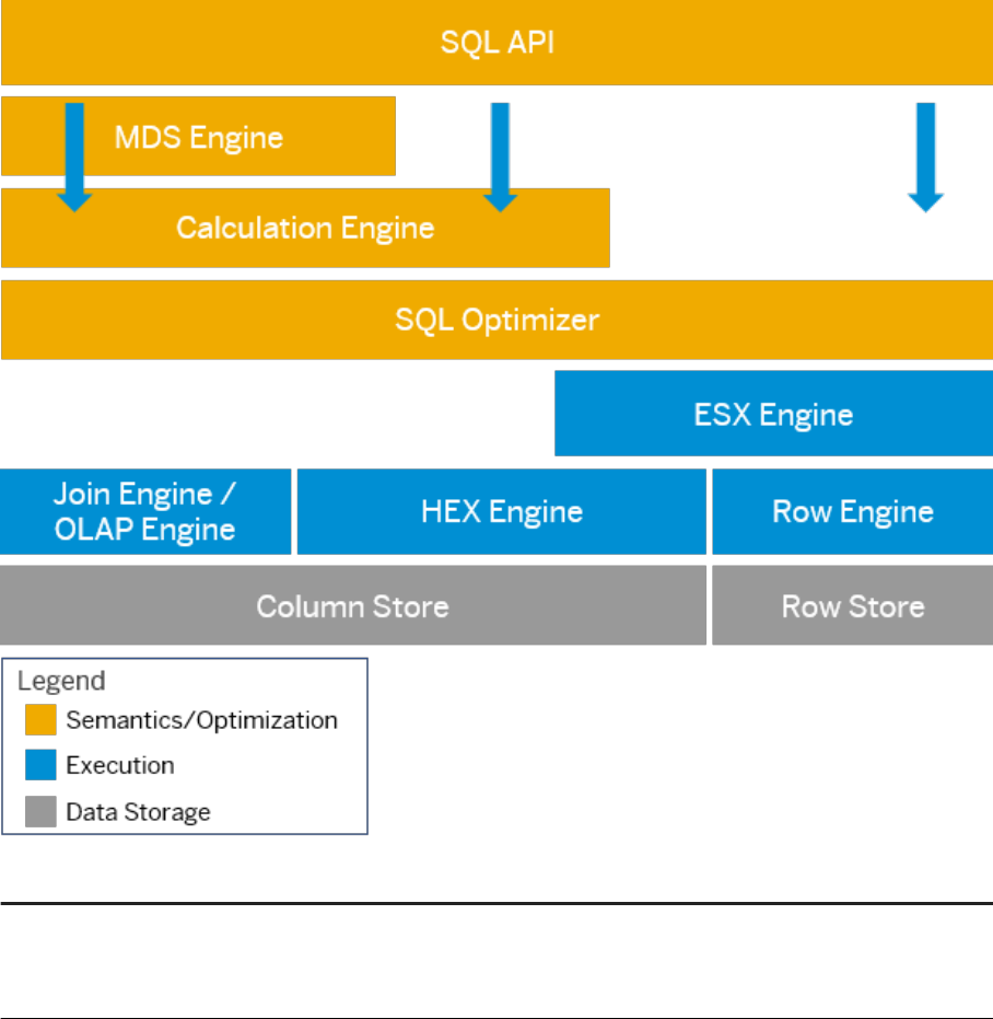
An overview of the SAP HANA query execution engines is shown below:
Engine
Description
HEX engine The SAP HANA Execution Engine (HEX) is a new engine that combines the func
tionality of other engines, such as the join engine and OLAP engine. Queries that
are not supported by HEX or where an execution is not considered benecial are
automatically routed to the former engine.
22 P U B L I C
SAP HANA Performance Guide for Developers
Query Execution Engine Overview
Engine Description
ESX engine The SAP HANA Extended SQL Executor (ESX) is a new frontend execution engine
that replaces the row engine in part, but not completely. It retrieves database re
quests at session level and delegates them to lower-level engines like the join en
gine and calculation engine.
Join engine
The join engine is used to run plain SQL. Column tables are processed in the join
engine.
OLAP engine The OLAP engine is primarily used to process aggregate operations. Calculated
measures (unlike calculated columns) are processed in the OLAP engine.
Calculation engine Calculation views, including star joins, are processed by the calculation engine. To
do so, the calculation engine may call any of the other engines directly or indi
rectly.
Row engine The row engine is designed for OLTP scenarios. Some functionality, such as par
ticular date conversions or window functions, are only supported in the row en
gine. The row engine is also used when plain SQL and calculation engine func
tions are mixed in a calculation view.
MDS engine
SAP HANA multi-dimensional services (MDS) is used to process multidimen
sional queries including aggregation, transformation, and calculation.
The queries are translated into an SAP HANA calculation engine execution plan or
SQL, which is executed by the SAP HANA core engines.
MDS is integrated with the SAP HANA Enterprise Performance Management
(EPM) platform and is used by reporting and planning applications.
The query languages currently supported use the Information Access (InA)
model. The InA model simplies the denition of queries with rich or even com
plex semantics. Data can be read from all kinds of SAP HANA views, EPM plan
data containers, and so on. The InA model also includes spatial (GIS) and search
features.
Related Information
New Query Processing Engines [page 24]
Changing an Execution Engine Decision [page 126]
SAP HANA Performance Guide for Developers
Query Execution Engine Overview
P U B L I C 23
4.1 New Query Processing Engines
Two new processing engines to execute SQL queries are being phased in to SAP HANA (applicable as of SAP
HANA 2.0 SPS 02). The new engines are designed to oer better performance, but do not otherwise aect the
functionality of SAP HANA.
The new engines are active by default (no conguration is required) and are considered by the SQL optimizer
during query plan generation:
● SAP HANA Extended SQL Executor (ESX)
● SAP HANA Execution Engine (HEX)
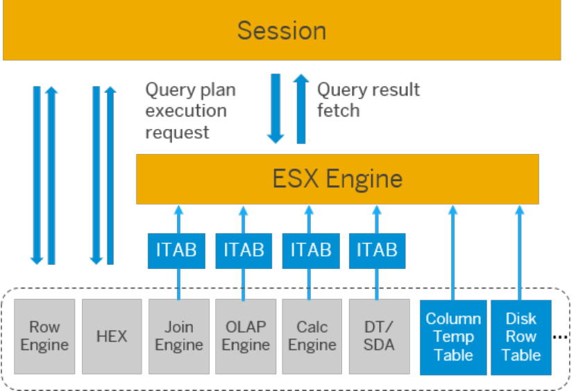
SAP HANA Extended SQL Executor (ESX)
The SAP HANA Extended SQL Executor (ESX) is a frontend execution engine that replaces the row engine in
part, but not completely. It retrieves database requests at session level and delegates them to lower-level
engines like the join engine and calculation engine. Communication with other engines is simplied by using
ITABs (internal tables) as the common format.
An overview is shown below:
24
P U B L I C
SAP HANA Performance Guide for Developers
Query Execution Engine Overview
SAP HANA Execution Engine (HEX)
The SAP HANA Execution Engine (HEX) is a query execution engine that will replace other SAP HANA engines
such as the join engine and OLAP engine in the long term, therefore allowing all functionality to be combined in
a single engine. It connects the SQL layer with the column store by creating an appropriate SQL plan during the
prepare phase. Queries that are not supported by HEX or where an execution is not considered benecial are
automatically routed to the former engine.
Related Information
ESX Example [page 25]
Disabling the ESX and HEX Engines [page 26]
4.2 ESX Example
Depending on the execution plan of a query, the SQL optimizer potentially replaces any operators that take
ITAB as an input with ESX operators, if this allows any unnecessary conversion between the column and the
row engines to be avoided.
The execution plans (with and without ESX) are shown below for the following query:
create column table c1 (a decimal(38), b int);
insert into c1 (select (element_number/20), to_int(mod(element_number,20)) from
series_generate_integer(1, 0, 100));
create column table c2 (a decimal(38));
insert into c2 (select row_number () over (partition by a order by b) from c1);
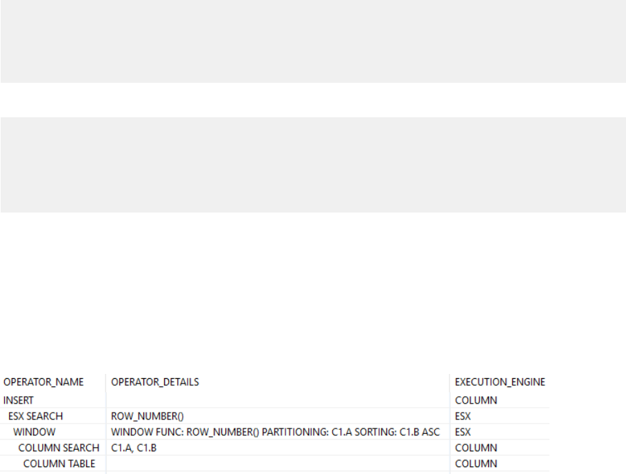
The standard execution plan (that is, without ESX) would be as follows:
INSERT COLUMN
C2C Converter COLUMN
WINDOW ROW
C2R Converter ROW
COLUMN SEARCH COLUMN
COLUMN TABLE COLUMN
In the above, the C2C Converter converts the row engine result to an ITAB, and the C2R Converter converts the
ITAB to a data structure that can be consumed by the row engine.
With ESX, however, the ESX WINDOW operator directly takes an ITAB as input and produces an ITAB as the
result, therefore allowing the unnecessary conversions to be skipped. The ESX engine also replaces non-row-
engine operators where the optimizer sees room for optimization, especially if this allows unnecessary
conversions to be skipped.
The ESX explain plan would be as follows:
SAP HANA Performance Guide for Developers
Query Execution Engine Overview
P U B L I C 25
4.3 Disabling the ESX and HEX Engines
You can disable and enable the engines using hints or conguration parameters. The engines should not be
disabled permanently because they are being actively developed and improved in each release.
Query Hints
You can use hints with queries to explicitly state which engine should be used to execute the query. For each
engine, two hint values are available to either use or completely ignore the engine. The following table
summarizes these and is followed by examples:
Hint value Eect
USE_ESX_PLAN Guides the optimizer to prefer the ESX engine over the standard engine.
NO_USE_ESX_PLAN Guides the optimizer to avoid the ESX engine.
USE_HEX_PLAN Guides the optimizer to prefer the HEX engine over the standard engine.
NO_USE_HEX_PLAN Guides the optimizer to avoid the HEX engine.
Sample Code
SELECT * FROM T1 WITH HINT(USE_ESX_PLAN);
SELECT * FROM T1 WITH HINT(NO_USE_HEX_PLAN);
Note that "prefer" takes precedence over "avoid". When hints are given that contain "prefer" and "avoid" at the
same time, "prefer" is always selected.
In the following, ESX_JOIN would be selected:
Sample Code
WITH HINT(NO_USE_ESX_PLAN, ESX_JOIN)
In the following, ESX_SORT would be selected:
Sample Code
WITH HINT(NO_ESX_SORT, ESX_SORT)
In the following, USE_ESX_PLAN would be selected:
Sample Code
WITH HINT(USE_ESX_PLAN, NO_USE_ESX_PLAN)
26
P U B L I C
SAP HANA Performance Guide for Developers
Query Execution Engine Overview

Conguration Parameters
If necessary (for example, if recommended by SAP Support), you can set conguration parameters to
completely disable the engines.
Each engine has a single parameter which can be switched to disable it:
File Section Parameter Value Meaning
indexserver.ini sql esx_level Default 1, set to 0 to
disable
Extended SQL executor enabled
indexserver.ini sql hex_enabled Default True, set to
False to disable
HANA execution engine enabled
Note
Disabling HEX using INI parameters can have a signicant impact on system behavior. The preferred
method is therefore to use HINT to specically reroute individual queries.
Related Information
Using Hints to Alter a Query Plan [page 126]
HINT Details
SAP HANA Performance Guide for Developers
Query Execution Engine Overview
P U B L I C 27

5 SQL Query Performance
Ensure your SQL statements are ecient and improve existing SQL statements and their performance.
Ecient SQL statements run in a shorter time. This is mostly due to a shorter execution time, but it can also be
the result of a shorter compilation time or a more ecient use of the plan cache.
This section of the guide focuses on the techniques for improving execution time. When execution time is
improved, a more ecient plan is automatically stored in the cache.
Related Information
SQL Process [page 28]
SAP HANA SQL Optimizer [page 31]
Analysis Tools [page 50]
Case Studies [page 83]
SQL Tuning Guidelines [page 116]
5.1 SQL Process
Although database performance depends on many dierent operations, the SELECT statement is decisive for
the SQL optimizer and optimization generally.
When more than one SELECT statement is executed simultaneously, query processing occurs for each
statement and gives separate results, unless the individual statements are intended to produce a single result
through a procedure or a calculation view. These separate but collectively executed statements also produce
separate SQL plan cache entries.
Note
The performance issues addressed here involve SELECT statements. However, they also apply to other
data manipulation language (DML) statements. For example, the performance of an UPDATE statement is
based on that of a SELECT statement because UPDATE is an operation that updates a selected entry.
28
P U B L I C
SAP HANA Performance Guide for Developers
SQL Query Performance
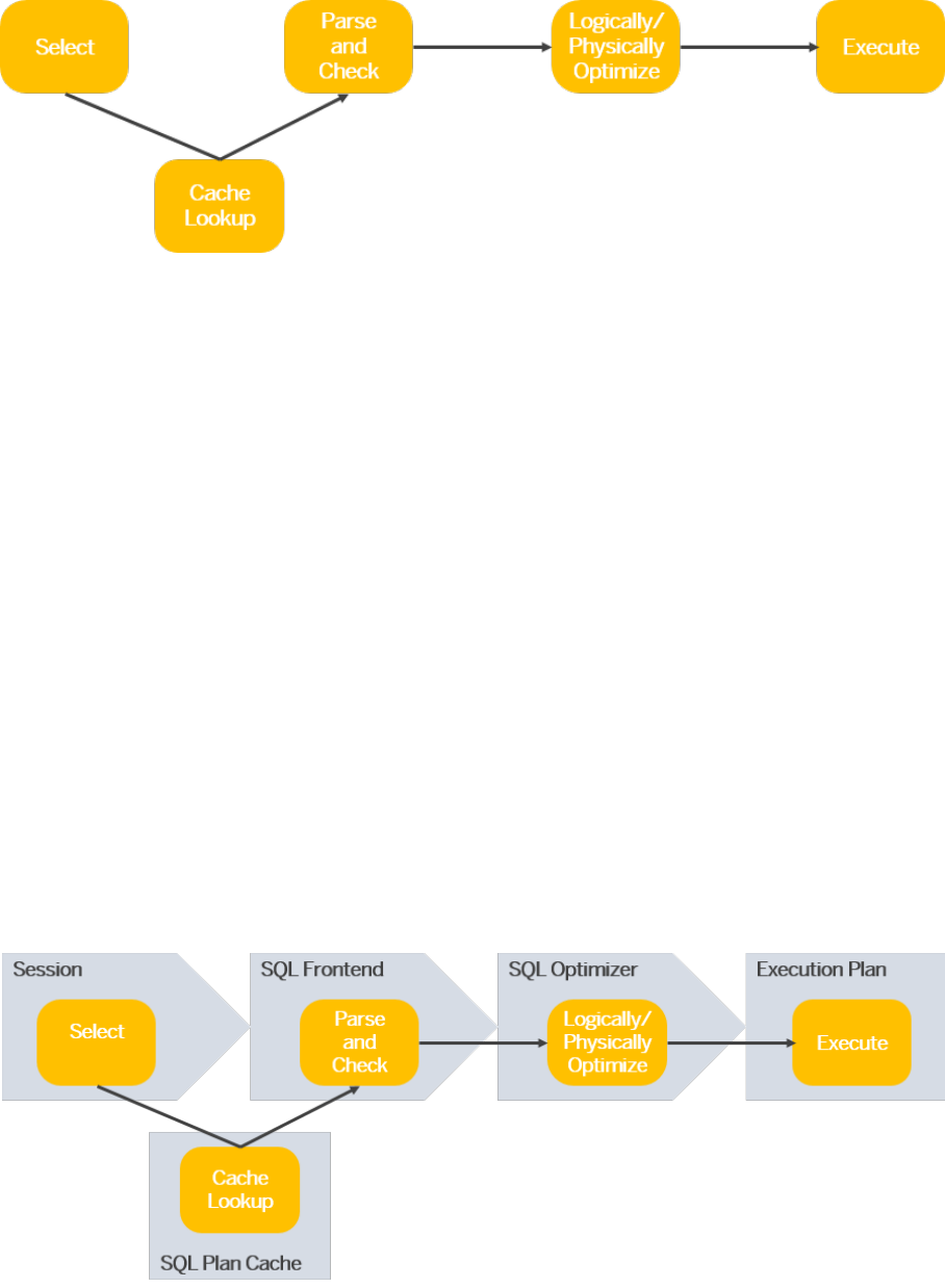
The SAP HANA SQL process starts with a SELECT statement, which is then looked up in the cache, parsed,
checked, optimized, and made into a nal execution plan. An overview is shown below:
The set of sequences to parse, check, optimize, and generate a plan is called query compilation. It is
sometimes also referred to as “query preparation”. Strictly, however, query preparation includes query
compilation because a query always needs to be prepared, even if there is nothing to compile. Also, query
compilation can sometimes be skipped if the plan already exists. In this case, the stored cache can be used
instead, which is one of the steps of query preparation.
When a SELECT statement is executed, the cache is rst checked to see if it contains the same query string. If
not, the query string is translated into engine-specic instructions with the same meaning (parsing) and
checked for syntactical and semantical errors (checking). The result of this is a tree, sometimes a DAG
(Directed Acyclic Graph) due to a shared subplan, which undergoes several optimization steps including logical
rewriting and cost-based enumerations. These optimizations generate an executable object, which is stored in
the SQL plan cache for later use.
Related Information
SQL Processing Components [page 29]
5.1.1 SQL Processing Components
The main components involved in processing an SQL query are the session, the SQL frontend, the SQL
optimizer, and the execution plan.
An overview is shown below:
SAP HANA Performance Guide for Developers
SQL Query Performance
P U B L I C 29
Session
The rst layer that a query passes through when it is executed is the session. A session is sometimes named
"eapi" or "Eapi".
The session layer is important because it is the rst layer in SQL processing. When you work with the SQL plan
cache or the dierent types of traces, you might need to consider the session layer. Also, when you work with
dierent clients, dierent sessions with dierent session properties are created. New transactions and working
threads are then created based on these.
SQL Frontend
The SQL frontend is where the SQL statement is parsed and checked.
When a statement is parsed, it is translated into a form that can be understood by the compiler. The syntax and
semantics of the executed statement are then checked. An error is triggered if the syntax of the statement is
incorrect, which will also cause the execution of the statement to fail. A semantic check checks the catalog to
verify whether the objects called by the SQL statement are present in the specied schema. Missing user
privileges can be an issue at this point. If the SQL user does not have the correct permission to access the
object, the object will not be found. When these processes have completed, a query optimizer object is created.
Query Optimizer
The query optimizer object, often referred to as a QO tree, is initially a very basic object that has simply
undergone a language translation. The critical task of the query optimizer is to optimize the tree so that it runs
faster, while at the same time ensuring that its data integrity is upheld.
To do so, the optimizer rst applies a set of rules designed to improve performance. These are proven rules that
simplify the logical algorithms without aecting the result. They are called "logical rewriting rules" because by
applying the rules, the tree is rewritten. The set of rewriting rules is large and may be expanded if needed.
After the logical rewriting, the next step is cost-based enumeration, in which alternative plans are enumerated
with estimated costs. Here, the cost is disproportionate to the plan’s performance. It is a calculated measure of
the processing time of the operator when it is executed by the plan. A limit is applied to the number of cost
enumerations, with the aim of reducing compilation time. Unlimited compilation time might help the optimizer
nd the best plan with the minimal execution time, but at the cost of the time required for its preparation.
While doing the cost enumeration, the optimizer creates and compares the alternatives from two perspectives,
a logical and a physical one. Logical enumerators provide dierent tree shapes and orders. They are concerned
with where each operator, like FILTER and JOIN, should be positioned and in what order. Physical enumerators,
on the other hand, determine the algorithms of the operators. For example, the physical enumerators of the
JOIN operator include Hash Join, Nested Loop Join, and Index Join.
30
P U B L I C
SAP HANA Performance Guide for Developers
SQL Query Performance
Executors
Once the optimization phase has completed, an execution plan can be created through a process called "code
generation" and sent to the dierent execution engines. The SAP HANA execution engines consist of two
dierent types, the row engine and the column engine.
The row engine is a basic processing engine that is commonly used in many databases, not only in SAP HANA.
The column engine is an SAP HANA-specic engine that handles data in a column-wise manner. Determining
which engine is faster is dicult because it always depends on many factors, such as SQL complexity, engine
features, and data size.
SQL Plan Cache
The rst and foremost purpose of SQL plan cache is to minimize the compilation time of a query. The SQL plan
cache is where query plans are stored once they pass the session layer, unless instructed otherwise.
Underlying the SQL plan cache is the monitoring view M_SQL_PLAN_CACHE.
The M_SQL_PLAN_CACHE monitoring view is a large table with primary keys that include user, session,
schema, statement, and so on.
To search for a specic cache entry or to ensure a query has a cache hit, you need to make sure you enter the
correct key values. To keep the table size to a minimum and to prevent it from becoming outdated, the entries
are invalidated or even evicted under specic circumstances (see SAP HANA Administration Guide). Therefore,
good housekeeping for the SQL plan cache involves striking a balance between cache storage size and frequent
cache hits. A big cache storage will allow almost all queries to take advantage of the plan cache, resulting in
faster query preparation, but with the added risk of an ineective or unintended plan and huge memory
consumption. Primary keys, the invalidation and eviction mechanism, and storage size settings are there for a
good reason.
Related Information
SAP HANA Administration Guide
5.2 SAP HANA SQL Optimizer
The two main tasks of the SQL optimizer are rule-based and cost-based optimization. The rule-based
optimization phase precedes cost-based optimization.
Rule-based optimization involves rewriting the entire tree by modifying or adding operators or information that
is needed. Every decision the optimizer makes must adhere to predened rules that are algorithmically proven
to enhance performance. Cost-based optimization, which consists of logical and physical enumeration,
involves a size and cost estimation of each subtree within the tree. The optimizer then chooses the least costly
plan based on its calculations.
SAP HANA Performance Guide for Developers
SQL Query Performance
P U B L I C 31
Note that rule-based optimization is a step-by-step rewriting approach applied to a single tree whereas cost-
based optimization chooses the best tree from many alternative trees.
The sections below describe each of the optimization steps. Rules and enumerators that are frequently chosen
are explained through examples. Note that the examples show only a subset of the many rules and
enumerators that exist.
Related Information
Rule-Based Optimization [page 32]
Cost-Based Optimization [page 36]
Decisions Not Subject to the SQL Optimizer [page 48]
Query Optimization Steps: Overview [page 49]
5.2.1 Rule-Based Optimization
The execution times of some query designs can be reduced through simple changes to the algorithms, like
switching operators or converting one operator to another, irrespective of how much data the sources contain
and how complex they are.
These mathematically proven rules are predened inside the SAP HANA SQL optimizer and provide the basis
for the rule-based optimization process. This process is very ecient and does not require data size estimation
or comparison of execution cost.
The frequently used rules are described in this section.
Related Information
Unfold Calculation View [page 33]
Select Pull-Up, Column Removal, Select Pushdown [page 34]
Simplify: Remove Group By [page 34]
Simplify: Remove Join [page 35]
Heuristic Rules [page 35]
How the Rules are Applied [page 36]
32
P U B L I C
SAP HANA Performance Guide for Developers
SQL Query Performance
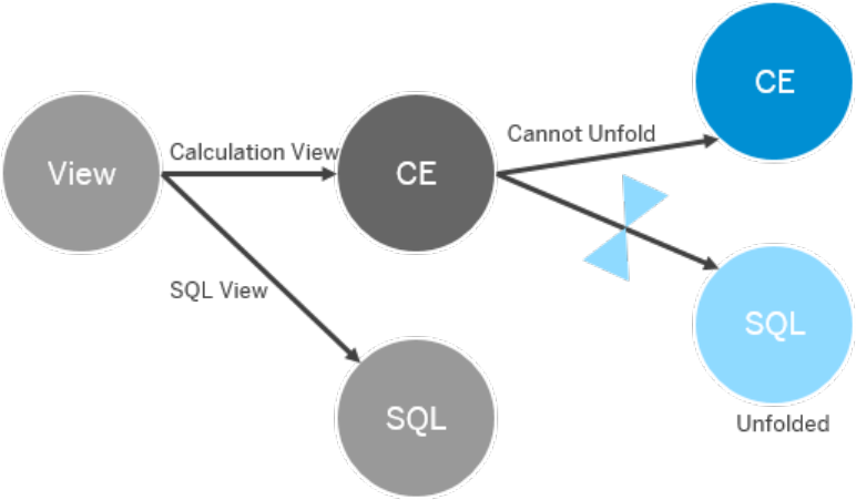
5.2.1.1 Unfold Calculation View
SQL is relational whereas calculation models are non-relational. To enable a holistic approach and integration
with the SQL optimizer, calculation models are translated into a relational form wherever possible. This is called
calculation view unfolding.
This process is shown below:
To understand calculation view unfolding, a good knowledge of calculation views is needed. A calculation view
is an SAP HANA-specic view object. Except for a standard SQL view that can be read with SQL, it consists of
functions in the SAP HANA calculation engine language, which are commonly referred to as "CE functions".
Due to this language dierence, the SQL optimizer, which only interprets SQL, cannot interpret a CE object
unless it is coded otherwise. Calculation view unfolding, in this context, is a mechanism used to pass
"interpretable" SQL to the SQL optimizer by literally unfolding the compactly wrapped CE functions.
Calculation view unfolding is always applied whenever there are one or more calculation views. This is because
it is more cost ecient to run the complete optimization process in one integrated optimizer, the SQL optimizer
in this context, than to leave the CE objects to be handled by the calculation engine optimizer.
Sometimes, however, the calculation view unfolding rule is blocked and the calculation engine needs to take
over the task. There are various unfolding blockers, ranging from ambiguous to straightforward. If a calculation
view is not unfolded and you think it should be, you can nd out more about the blocker by analyzing the traces.
Related Information
SQL Trace [page 68]
SQL Optimization Step Debug Trace [page 70]
SAP HANA Performance Guide for Developers
SQL Query Performance
P U B L I C 33
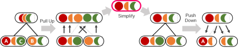
5.2.1.2 Select Pull-Up, Column Removal, Select Pushdown
The main purpose of compilation is to minimize execution time, which depends heavily on the level of
complexity. The major cause of increased complexity is redundant column projection.
As part of query simplication, the optimizer pulls all projection columns up to the top of the tree, applies
simplication measures, which include removing unnecessary columns, and then pushes down the lters as far
as possible, mostly to the table layer, as shown below:
This set of pull-up, remove, and pushdown actions can be repeated several times during one query compilation.
Also, the simplication in between the pull-up and pushdown actions may include other measures like adding
more lters, removing operators, or even adding more operators to make optimization more ecient. The
query plan might temporarily be either shorter or longer while the later optimization steps are being compiled.
Related Information
SQL Optimization Step Debug Trace [page 70]
5.2.1.3 Simplify: Remove Group By
A tree might have multiple aggregation operators one after the other. This might be because you intended it, or
because the plan was shaped like this during logical rewriting.
For example, after aggregating the rst and second columns, another aggregation is done for the third column,
and lastly the fourth and fth columns are also aggregated.
While a query like this does not seem to make much sense, this type of redundant or repeated aggregation
occurs frequently. It mainly occurs in complex queries and when SQL views or calculation views are used. Often
users don’t want to use multiple data sources because they are dicult to maintain. Instead they prefer a single
or compact number of the views that can be used in many dierent analytical reports. Technically, therefore,
the views need to be parameterized with dynamic variables, which means that the query plans can always vary
according to the actual variable values. Also, for maintenance purposes, users don’t create all views from
scratch, but instead reuse existing views as a data source for another view. Therefore, by the time the query is
34
P U B L I C
SAP HANA Performance Guide for Developers
SQL Query Performance
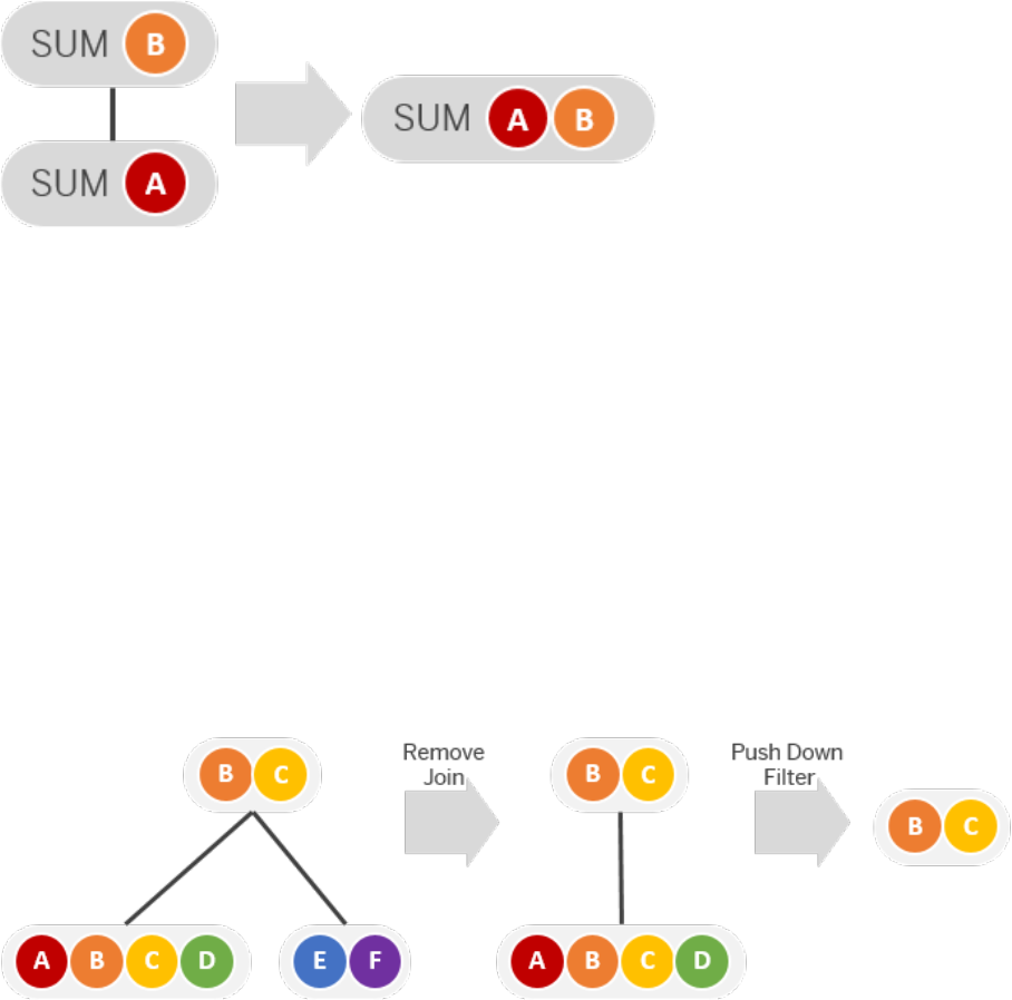
made into a logical plan through calculation view unfolding, column pushdown, and redundancy removal, the
aggregations might be stacked, as shown in the example below:
To tackle this redundancy, the SQL optimizer removes or simplies the aggregation operators by turning them
into a single operation, unless there are limiting factors. If the child aggregation does not contain all the GROUP
BY columns that are dened for its parent, their aggregations cannot be merged. Also, if the parent has
aggregation functions other than MIN, MAX, or SUM, which makes the parent aggregation itself rather heavy,
the aggregations cannot be merged.
5.2.1.4 Simplify: Remove Join
A join can be simplied when there is a logical redundancy.
One example would be a join that only needs the columns from one of the join children. In this case, no columns
are needed from the other child, so there is no need to do the join. Therefore, the join is removed and there is
just a projection. The example below shows how there will eventually be just one operator, for example one
projection or one table scan:
5.2.1.5 Heuristic Rules
The predened optimization rules include heuristic rules. Heuristic rules are not directly derived from
mathematical or algorithmic calculation, but from numerous examinations and analyses.
For example, when join children contain so much data that their size exceeds a certain threshold, it is known
that this is very inecient. It is also known that in these cases performance can be improved by changing the
join order, that is, by switching the join with another join in the lower layer. The decisive factor for this
optimization rule is the threshold, because it determines whether the rule is valid and should therefore be
applied. One record less can result in a completely dierent result. Heuristic results, therefore, have advantages
SAP HANA Performance Guide for Developers
SQL Query Performance
P U B L I C 35
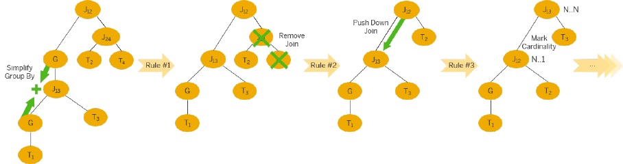
and disadvantages. On the one hand, they can signicantly improve performance through simple changes, but
on the other hand, they can result in an undesirable and un-optimized decision.
Heuristic rules are one of the most prominent root causes of performance issues. There are still quite a few
cases that could be solved simply by limiting the optimization level to non-heuristic rules. But most of the time,
query performance benets from heuristic rules. Therefore, heuristic rules should not be ignored but they must
be carefully observed when there is a performance issue.
5.2.1.6 How the Rules are Applied
The algorithms of the optimization rules are predened as well as the order in which they are applied. The SQL
optimizer goes through the list of rules row by row to check if the rule is applicable. Applicable rules apply,
others don't.
The example below shows the application of a series of rules:
As shown above, rule-based optimization is sequential rather than concurrent. This is worth noting because
cost-based optimization (see below) is essentially a concurrent task.
Some rules are applied repeatedly until a specic condition is satised, and sometimes one rule triggers
another one, although this is not necessarily a prerequisite for every query. The rules are repeatedly applied to
the same plan tree, modifying the tree in every step, until the list of predened rules has been completed and
the SQL optimizer can move on to the next step, which is cost-based optimization.
Related Information
Cost-Based Optimization [page 36]
5.2.2 Cost-Based Optimization
Cost-based optimization involves nding the optimal plan by analyzing and comparing execution costs. Costs
are acquired by mathematically evaluating sizes. In this context, size basically indicates the number of the rows
in the dataset, but it can also be larger depending on the data type and operator.
A table with a hundred million records is not that big for a commercial database. However, if it has multiple text
columns like DOUBLE or TEXT, and if there is a window function like ROW_NUMBER or RANK that requires row-
36
P U B L I C
SAP HANA Performance Guide for Developers
SQL Query Performance
wise evaluation on those columns, the plan will no longer be clearly structured, and this will increase the costs.
In this example, the optimizer will try to minimize the intermediate result by pushing down the lters and joins
so that the row engine does not have to do the window function evaluation on a massive amount of data.
In a comparative sense, rule-based optimization can be regarded as broad macroscopic work, whereas cost-
based optimization is more like delicate microscopic work. Rule-based optimization is relatively predictable
and sometimes even obvious because the rules are predened and work in a set way. Nevertheless, those rules
cannot address every detail of an individual query. So, cost-based optimization, as an atomic assessment
process that tags each operator with its size and cost, adds more accuracy to the performance optimization.
Enumeration Types
There are two types of enumeration, logical enumeration and physical enumeration. Logical enumeration is
used to build the overall shape of the tree. Physical enumeration is used to determine the characteristics of
each of its components.
The only goal of the SQL optimizer is to achieve eciency, and since its main aim is to minimize execution time,
it is often prepared to sacrice available resources such as memory and CPU for this purpose. This in turn can
raise other performance issues, such as the out-of-memory (OOM) condition, which is described in a dedicated
section.
Related Information
Logical Enumeration [page 37]
Physical Enumeration [page 40]
Column Search [page 43]
How Enumeration Works [page 47]
5.2.2.1 Logical Enumeration
For the SAP HANA SQL optimizer, logical enumeration involves comparing the costs of all possible candidates
detected within the limited boundary of the search area. It includes proposing alternatives for each operator,
calculating the estimated costs, and deciding for or against that alternative depending on the costs.
Logical enumeration, therefore, is an enumeration of the format of the tree and a decision on the existence and
order of the operators. When a lter, join, or aggregation is pushed down through another operator, that is
where the logical enumerator has come into play. Usually, whenever something is pushed down through or into
something else, it is due to the logical enumerator. Cost is the key factor that determines the optimized logical
plan.
SAP HANA Performance Guide for Developers
SQL Query Performance
P U B L I C 37
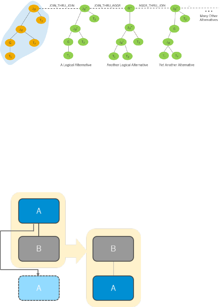
An example is shown below:
Related Information
_THRU_ [page 38]
PRE…_BEFORE_ [page 39]
5.2.2.1.1 _THRU_
Enumerators that belong to this category include JOIN_THRU_JOIN, JOIN_THRU_AGGR, and
LIMIT_THRU_JOIN. These A_thru_B enumerators literally move the rst operator A through the second B, and
position A below B in the plan tree. This is particularly eective when A reduces the data more than B does.
A_thru_B:
38
P U B L I C
SAP HANA Performance Guide for Developers
SQL Query Performance
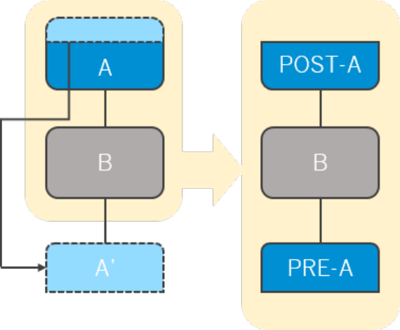
For example, suppose that there is an aggregation over a join, and this join is very heavy because it is a left
outer join with range join conditions on multiple timestamp columns. The SQL optimizer will try to push the
aggregation through the join so that it can reduce the dataset of one of the join candidates. This is
AGGR_THRU_JOIN. Pushing down operators like limit and lter also work within this context.
JOIN_THRU_JOIN basically switches the order of the joins. How eective this is will depend on the data sizes
involved. However, it does not negatively impact performance. Unlike rule-based rewriting, cost-based
optimization does not “change” anything until it reaches the optimized point or is limited by the enumeration
limit. During the process of enumeration, it tries out the enumeration rules and uses them to propose better
alternatives, which then are evaluated in terms of costs, allowing the most inexpensive plan to nally be
selected.
5.2.2.1.2 PRE…_BEFORE_
The most well-known enumerator of this type is PREAGGR_BEFORE_JOIN. PREAGGR_BEFORE_JOIN is a
preaggregation. This means that it adds a preaggregation to one of the join candidates, so that the size of the
join can be reduced. In these cases, the aggregation over the join is called "post-aggregation".
PREAGGR_BEFORE_JOIN:
If you want to do a preaggregation on both children of the join, you can use
DOUBLE_PREAGGR_BEFORE_JOIN.
SAP HANA Performance Guide for Developers
SQL Query Performance
P U B L I C 39
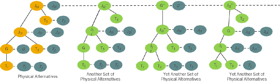
5.2.2.2 Physical Enumeration
Physical enumeration is similar to logical enumeration. However, while logical enumerators help generate
alternatives with a dierent logical structure and order of the operators, physical enumerators enumerate the
engine options, operator types, execution locations, and so on.
For example, in the physical enumeration phase, physical enumerators determine whether the column engine
or the row engine should perform a certain operation. They also determine whether a hash join, nested loop
join, index join, or other type of join should be used.
Physical alternatives:
Related Information
CS_ or RS_ [page 40]
Cyclic Join [page 41]
REMOTE_ [page 42]
5.2.2.2.1 CS_ or RS_
CS and RS denote column store and row store. This applies in SAP HANA generally and not just in the SQL
optimizer. Any enumerators that start with CS indicate that column engines should be used rather than row
engines for the designated operation.
For example, CS_JOIN means that a join should be performed with column engines. However, this is still
subject to the principle of cost-based optimization, which ensures that the most inexpensive plan is selected as
the nal plan. Therefore, there is no guarantee that the joins in this plan would be performed in column engines,
even if you were to use a hint to try to enforce it. The joins will ultimately only be handled by column engines if
the cost evaluation conrms that CS_JOIN is expected to give a better outcome.
40
P U B L I C
SAP HANA Performance Guide for Developers
SQL Query Performance
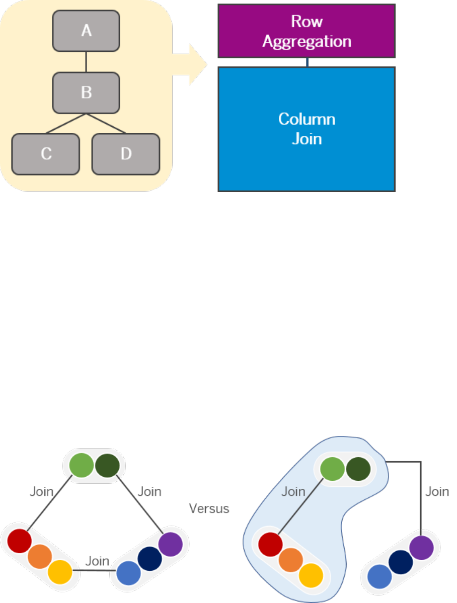
For example:
For information about which of the three main column engines (join, OLAP, or calculation engine) is responsible
for an operation, you need to examine traces such as the Explain Plan and Plan Visualizer, which show the nal
execution plan rather than the compilation procedure.
5.2.2.2.2 Cyclic Join
When three or more tables are joined together in a chain or cycle of joins, this is called a cyclic join. For
example, table A is joined with table B, which is joined with table C, and table C is joined with table A.
In SAP HANA, the cyclic inner join is natively supported by the column engines whereas the cyclic outer join is
not. So, when a cyclic join has outer joins, the cycle is broken into two parts. The join between table A and table
B is done rst, and its result is then joined with table C, or something similar. Determining which of the three
joins should be broken is a mathematical problem that the optimizer solves during compilation. The calculation
is based on the estimated size and costs of the joins. This approach does not present a problem.
A cyclic join broken into two parts:
The problem is when the cyclic join is an inner join. Because the column engines natively support it, the SQL
optimizer needs to decide whether to leave the cyclic join intact or whether to break it. Due to uncertain size
SAP HANA Performance Guide for Developers
SQL Query Performance
P U B L I C 41
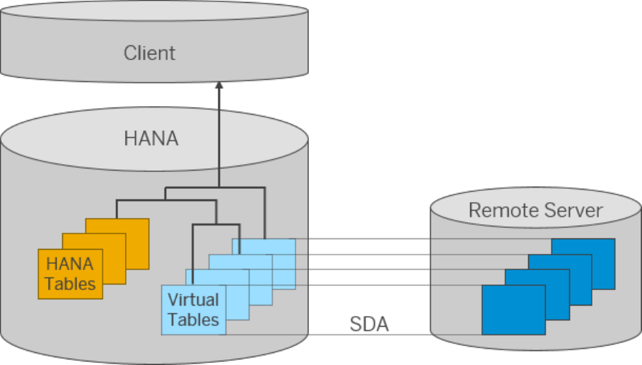
and cost estimations, and the unpredictable performance of the execution engines, the SQL optimizer
sometimes makes a bad decision, which in turn causes a performance issue. The issue is even more critical
when the data sizes of the children of the joins are large, because the materialized intermediate result is likely
to be huge.
Therefore, in cases where there are many complicated join relations, it is worth checking if there is a cyclic join
and if the cycle is broken. If the performance hot spot proves to be the cyclic join, one of the workarounds could
be to break it using the SQL hint NO_CYCLIC_JOIN. This indicates that breaking the cyclic join is preferable to
keeping it.
5.2.2.2.3 REMOTE_
This physical enumerator is used and only makes sense when there is a remote server connected to SAP
HANA.
Many companies use SAP HANA as an analytics database while they store their source data in another
database connected to the SAP HANA system. Examples of remote connections include Smart Data Access
(SDA), Near Line Storage (NLS), and Dynamic Tiering.
A connection to a remote server:
When a query containing a table from a remote server is compiled, table statistics are collected from the
remote server and used for cost estimation during cost-based enumeration.
As one of the physical enumeration processes, the SQL optimizer compares the costs of doing operations on
the remote server and on SAP HANA. For example, it evaluates what the cost would be to do a join on the
remote server and transmit its result to SAP HANA, and then compares it with the cost of transmitting the
whole data source to SAP HANA and running the join on SAP HANA. The network performance between SAP
HANA and the remote server can make this task more dicult.
42
P U B L I C
SAP HANA Performance Guide for Developers
SQL Query Performance
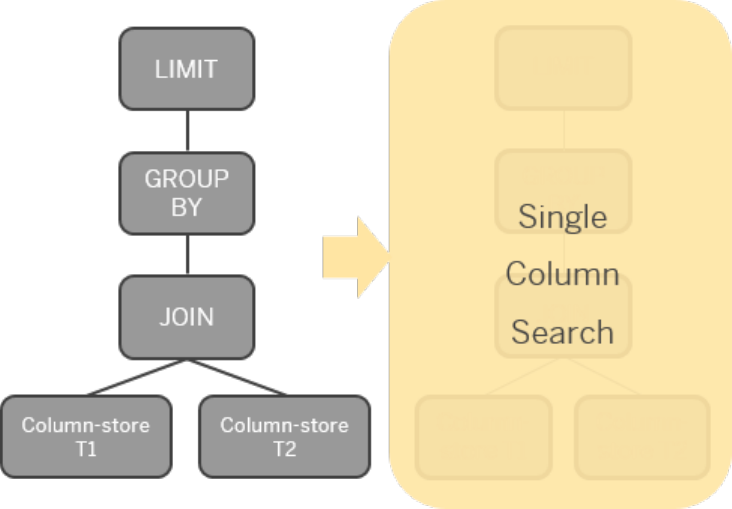
In terms of the remote execution, there can be quite a big dierence between what SAP HANA expects the
remote server would do and what it actually does. For example, according to the SQL optimizer’s plan, the
ltered data is supposed to be loaded from the remote server to SAP HANA. However, due to limited network
bandwidth and the huge volume of data, a performance issue may arise. An out-of-memory (OOM) situation
can also occur if there is not enough memory on the remote server. Therefore, when there is a remote server
involved in a query execution and the execution fails or runs slowly, you need to consider whether it might be
caused by the execution on the remote server. To do so, you need to examine the query statement transmitted
to the remote server to see how much time it took to run it and fetch the result.
5.2.2.3 Column Search
Column search is a composite operator that can be operated in a single IMS search call. An IMS search call is a
request from the SQL engine to the column engine, generally with the query execution plan (QE).
Each query plan that is passed to the column engines uses this interface. For an IMS search call to occur, the
query plan must have a columnar plan. A single IMS search call means that the SQL engine does not have to
send multiple execution request through IMS. Because the column search is composite, by denition, the
request can contain more than one operator, even though it is a single interface call.
A column search is created or decided on during cost-based physical enumeration. The decision to run a
column search is called “column search availability”. When a column search is “available”, it means that one or
more operators will be executed in column engines and that this operation will involve a single API call. For
example, a query has two column tables with JOIN, GROUPBY, and LIMIT operators in a bottom-up order.
Because the base tables are column-store table and the operators are natively supported by the column
engines, this query plan is likely to have at least one column search. If the optimizer decides that all three
operators can be combined into one composite operator, everything will be packed or absorbed into one single
column search, resulting in a fully columnar plan.
Single column search:
SAP HANA Performance Guide for Developers
SQL Query Performance
P U B L I C 43
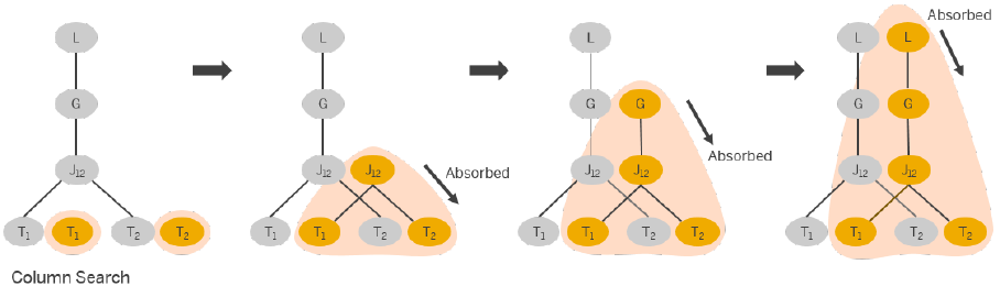
Related Information
Absorption [page 44]
Pushdown Blocker [page 45]
Singular Versus Stacked Column Search [page 46]
5.2.2.3.1 Absorption
Absorption is a mechanism that extends the column search boundary across the operators. Starting with the
table, the column search moves up along the tree and merges the operators, until it meets a blocker that
prevents its expansion.
The procedure by which the operators are merged into the column search is referred to as absorption. This is
shown below:
So that the operators can be absorbed into a column search, they should be types that are natively supported
by at least one of the column engines in SAP HANA.
For example, let's assume the JOIN is a range join that requires row-wise comparison. Because this join is not
natively supported by the column engines, it cannot be absorbed even though the join candidates are both
column-store tables. Because this join has already broken the column search, it is highly likely that the
aggregation and limit operations above it will be executed in row engines.
Now let’s assume that the join is an equi-join, which is natively supported by the column engines. The
aggregation above it, however, is very expensive when it is executed in column engines. Generally, this is due to
the expressions or calculated columns inside the aggregation. This aggregation operator, therefore, cannot be
absorbed into the column search, not because it is not supported, but because the plan would be more
expensive than without absorption.
There are also cases where operators cannot be merged into the column search due to their logical order, even
though they are natively supported by the column engines. For example, if the logical plan has an aggregation
that is then joined with another table, this join cannot be absorbed because this type of composite operator
that handles an aggregation rst and then a join is not supported by any of the column engines. Column
engines do support an aggregation over a join or a join over a join, but not a join over an aggregation. So, in this
case where there is a join over an aggregation, the column search will be divided into two searches, a column
search for the aggregation and possibly another column search containing the join above it.
44
P U B L I C
SAP HANA Performance Guide for Developers
SQL Query Performance
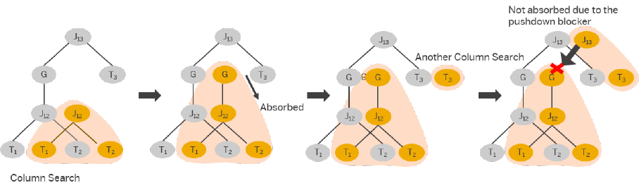
A column search with a join that cannot be absorbed:
When a column search is split into multiple parts, it is referred to as a stacked column search. A stacked
column search can signicantly impact the performance of the entire query.
Note that if the SQL optimizer decides that the join should be executed in a row engine rather than a column
engine, this will not be a stacked column search because there is only one column search and the operators
that are not absorbed will be handled in row engines.
Absorption, therefore, can only occur if an operator is natively supported by a column engine and if it is
expected to give a better result. Absorption occurs in a bottom-up manner and in a predened order until a
blocker is encountered. A valid order is as follows: Table scan – Join – Aggregation – Limit/Top.
5.2.2.3.2 Pushdown Blocker
A pushdown blocker is anything that prevents the absorption of an operator into an existing column search.
From a performance perspective, it is nearly always better to push down heavy operators, as is the case when
they are pushed down into the column search. However, pushdown blockers interfere with the pushdown
process.
Pushdown blockers are usually derived from the materialization operator and the limitations of the execution
engines. Some examples of blockers include the range join, window operators, limit/top, and logical order. The
best way to nd out which pushdown blockers are involved is to analyze the traces, particularly the SQL
Optimization Step trace.
Related Information
SQL Optimization Step Debug Trace [page 70]
SAP HANA Performance Guide for Developers
SQL Query Performance
P U B L I C 45
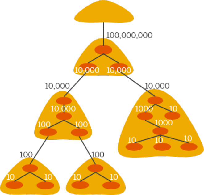
5.2.2.3.3 Singular Versus Stacked Column Search
A stacked column search is where there are multiple column searches stacked on top of each other. The Plan
Visualizer provides the most intuitive way to understand the stacked column search, while other traces also
provide similar information.
A stacked column search impacts SQL performance because it entails data materialization. Data
materialization is an operation where the intermediate result is converted into a physical temporary table, with
or without metadata information, and part of the physical memory is used to temporarily store the data. Its
memory consumption increases as the size of the intermediate data grows. In many out-of-memory (OOM)
cases, it has been found that a large part of memory is allocated for data materialization during a join. Even for
non-OOM performance issues, materialization of a vast amount of data normally takes a long time.
For example, consider the following:
The more complex a plan is, the more column searches that are stacked. Each column search can be regarded
as a data materialization operator. In the example, 8 base tables are used, and each table has no more than 10
rows. However, joined together, there are 100 million intermediate records. This number is not a problem for a
normal database, but it is a problem when so many records need to be physically stored in memory, even if it is
temporary. It becomes even more problematic if the intermediate result contains long texts such as TEXT,
BLOB, CLOB, and so on.
Because you can predict how the SQL optimizer will handle a query, you can prevent a plan from becoming a
stacked column search. The rst step is to remove the potential pushdown blockers and add as many lters as
possible to the data sources. Because SAP HANA is evolving, it is dicult to know exactly which pushdown
blockers there are. Nevertheless, there are several examples you can safely use as a preventive measure or
performance tuning method.
46
P U B L I C
SAP HANA Performance Guide for Developers
SQL Query Performance
Note, however, that despite these problems, you should not simply switch to row engines. Column engines are
by nature faster than row engines when massive data needs to be processed for analytical purposes.
Considering that most of the business data for heavy analytics is stored in column-store tables, fully columnar
plans will outperform row engines, with a few exceptions. However, it is important that you try to keep column
search stacks to a minimum. Due to their memory consumption, they can be critical for an in-memory
database and even lead to out-of-memory conditions. Therefore, you need to be aware of data materialization
when you use SQL, particularly where the intermediate results like join outputs are expected to be heavy. When
analyzing SQL, it is recommended that you try to identify problematic materialization and avoid it if possible by
using static lters or a union instead.
5.2.2.4 How Enumeration Works
Logical and physical enumerations are neither separate nor sequential processes. They are simultaneous and
continuous.
After rule-based optimization, the tree has been rewritten according to the predened rules that are applicable
to it. As it moves on to the enumeration process, an empty bucket called a "search space" is created, which will
store all the tree’s alternatives. Starting with the tables at the bottom of the tree, the SQL optimizer
investigates each node’s logical alternative. For example, for a simple base tree consisting of a join with an
aggregation above it, the logical enumerator AGGR_THRU_JOIN can create a logical alternative where the
aggregation is positioned below the join. Directly after this, the SQL optimizer tags the applicable physical
operators to each node. Examples for the join operation include Hash Join, Nested Loop Join, and Index Join.
Due to the physical operators that have been added, there are now multiple alternative plans to the original
plan. Each alternative is evaluated based on its costs, and only the least expensive ones are retained (the
others are pruned away). Having completed the work at the bottom of the tree, the optimizer moves on to the
upper nodes, for example, a lter, limit, or possibly another aggregation or join that is positioned above the join
and aggregation (base tree) already described. Then, logical alternatives and physical alternatives are created
on these nodes, the costs estimated, and pruning applied. This round of activities is repeated from the bottom
node up to the top.
SAP HANA Performance Guide for Developers
SQL Query Performance
P U B L I C 47
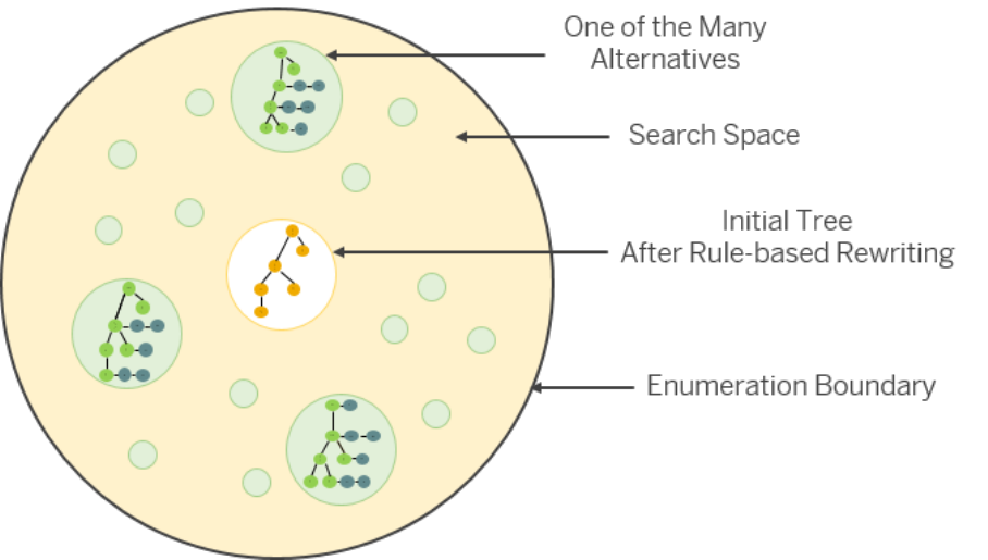
An enumeration limit is in place to ensure that the plan does not become too complex. By default, the
enumeration limit is 2,000. This means that the maximum number of alternatives the optimizer can create
during enumeration is 2,000. This is shown as the "Enumeration Boundary" below:
Although it is generally benecial to have a limit on the number of enumerated alternatives, it can sometimes
be disadvantageous. This might be the case when the optimizer fails to nd the optimal plan simply because
the optimal point is too far away, so the enumeration limit is reached rst, and compilation completed. In this
case, the result of the compilation is inecient and slow, which leads to another type of performance issue.
5.2.3 Decisions Not Subject to the SQL Optimizer
When cost-based enumeration ends, the nal query execution plan is generated (called “code generation”).
This is the plan that will be executed by the execution engines. At this point, the role of the SQL optimizer also
ends.
After code generation, the query plan can still be changed, but only by the execution engines. This is called
"engine-specic optimization" because the changes are determined and made by the execution engines.
Engine-specic decisions vary from engine to engine. An example of an engine-specic decision is the parallel
thread decision made by the join engine. During the optimization process, the SQL optimizer does not consider
aspects related to memory management and CPU. Its primary task is to make the plan run faster, and to do so
it uses all available resources to a maximum. Whether the query should run on multiple threads is not part of its
decision making. It is the join engine that is responsible for making this decision. This is also the reason why
you need to use an engine-specic hint, and not an SQL optimizer hint, to enforce parallel execution for the
query.
48
P U B L I C
SAP HANA Performance Guide for Developers
SQL Query Performance
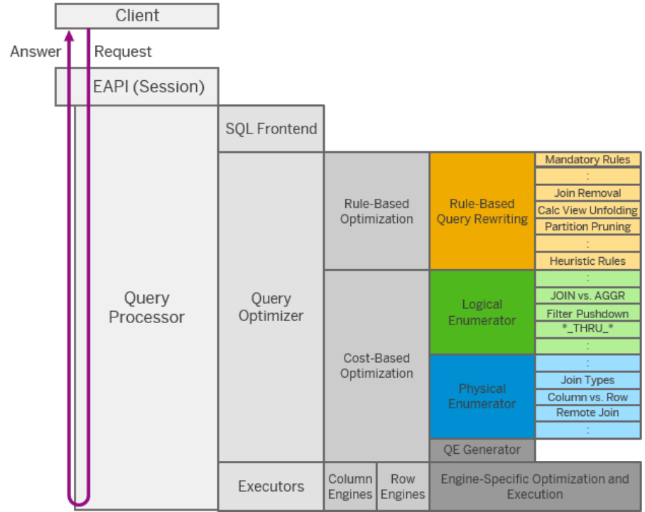
Related Information
HINT Details
5.2.4 Query Optimization Steps: Overview
The key to solving a performance issue is to nd the hot spot. This is the point at which the compilation
process no longer runs in an expected manner. To be able to identify the underlying issues, you require a
thorough understanding of the query optimization steps.
You need to know the specic activities that happen during each step of the query optimization process, as well
as the other activities that occur in the previous and next steps. This will allow you to pinpoint the root cause of
the problem and device a workaround.
An overview of the entire process is shown below:
SAP HANA Performance Guide for Developers
SQL Query Performance
P U B L I C 49

5.3 Analysis Tools
This section provides an overview of the tools and tracing options that are available.
Related Information
SQL Plan Cache [page 50]
Explain Plan [page 54]
Plan Visualizer [page 60]
SQL Trace [page 68]
SQL Optimization Step Debug Trace [page 70]
SQL Optimization Time Debug Trace [page 77]
Views and Tables [page 82]
5.3.1 SQL Plan Cache
The SQL plan cache is where the plan cache entries are stored for later use. Each time a query is executed, the
SQL plan cache is checked to see if there is a cached plan for the incoming query. If there is, this plan is
automatically used.
This means that generally you do not need to search for a cache as part of ordinary database administration.
However, when you have experienced slow query execution and you need to access it and its statistics, the SQL
plan cache is where you should look.
Finding an entry in the SQL plan cache can be dicult because the table contains many primary keys. However,
a query is usually always executed in the same client with the same user. In daily business, it is generally the
same person who logs into a system with the same user account and runs the same report in the same
manner. So, if all this applies, it is not very dicult to nd the cache. You simply need to set a lter, which
contains part of the query that you always use, on the STATEMENT_STRING column. You will then get a single
cache entry that has recently been used for repeated executions.
The diculty arises when there are many users that run the same or similar statements from many dierent
client environments with dierent variables from dierent schemas. In these cases, you rst need to know
which of those variants has caused the performance issue that you are analyzing. Otherwise, you will have to
manually go through multiple lines of search results from M_SQL_PLAN_CACHE to nd the entry that you are
looking for.
You can search the SQL plan cache using an SQL statement like the following:
SELECT
"STATEMENT_STRING", "IS_VALID", "LAST_INVALIDATION_REASON", "STATEMENT_HASH",
"USER_NAME", "IS_VALID", "PLAN_ID", "EXECUTION_COUNT", "PREPARATION_COUNT",
"LAST_EXECUTION_TIMESTAMP", "LAST_PREPARATION_TIMESTAMP"
FROM "M_SQL_PLAN_CACHE"
WHERE "STATEMENT_STRING" LIKE '%<part of your statement>%'
AND "HOST" = '<host_name>'
50
P U B L I C
SAP HANA Performance Guide for Developers
SQL Query Performance
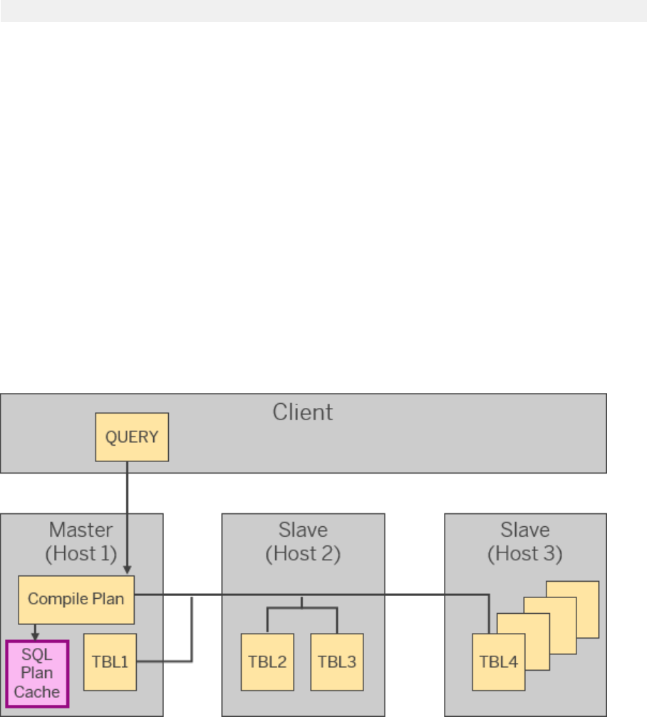
AND "USER_NAME" = '<database user name>';
5.3.1.1 HOST
The host matters particularly when the tables used as data sources are partitioned and distributed across the
hosts. This is because of the way in which the SQL plan cache integrates multiple physical tables that are host-
dependent and reside separately.
In other words, dierent cache entries are stored when the same query is compiled on host A and when it is
compiled on host B. The plan compiled on host A is stored in host A with value "A" in the HOST column, and the
plan compiled on host B is stored in host B with "B" in the HOST column. Later, when M_SQL_PLAN_CACHE is
called from any of the hosts, both records appear in the result. In addition, the location of the compilation is
decided on demand by the statement routing rules when the query is executed.
Since this is the underlying mechanism of the SQL plan cache, you will get double, triple, or even more records
when you search the M_SQL_PLAN_CACHE monitoring view using only the statement string lter. Therefore,
host information is important to nd the correct entry.
An example with multiple hosts and distributed tables is shown below:
5.3.1.2 USER_NAME and SCHEMA_NAME
Dierent entries are stored in the plan cache for dierent execution users. This aects the cache hit ratio when
the identical query is repeatedly executed by multiple users.
If there are no cash hits for your query but you are sure there should be, it is highly likely that you have logged in
with another user, for example, "TRACE_USER" or "ADMIN_USER" for tracing or administration tasks, while the
cache might have been compiled by one of the business users like "SAPABAP1" or "SAPPRD".
SAP HANA Performance Guide for Developers
SQL Query Performance
P U B L I C 51
To ensure you have a cache hit, you must log in with the user experiencing the performance issue or long-
running threads. To search for one specic query plan in the SQL plan cache, you should set a user lter as well
as a schema lter.
5.3.1.3 SESSION_PROPERTIES
Dierent clients create dierent cache entries. This is controlled by the SESSION_PROPERTIES column. The
session property contains session context information, including the client interface, client type, and client
number.
This means, for example, that dierent entries are created when the same query is run from the SAP HANA
SQL console and from another BI analytics client. These entries might also have dierent users. Therefore, if
you are not certain which application or execution has caused the issue and you search using a single
STATEMENT_STRING, you should expect multiple search results.
5.3.1.4 STATEMENT_STRING
STATEMENT_STRING is the best known and most popular search criterion in the SQL plan cache because it is
intuitive and simple to use.
STATEMENT_STRING is handy because you can usually recall at least a few column names, or the table, view,
or procedure name used in the FROM clause directly after executing the query. In fact, "STATEMENT_STRING
LIKE '%<part-of-the-statement>%'" is a favorite among query tuning experts. However, it is worth
remembering that a microscopic approach through ltering other columns like user, schema, host, and client
can reduce the search time and make your work more accurate.
5.3.1.5 IS_VALID
For maintenance purposes, SQL plan cache entries can be invalidated or evicted.
Evicted plans no longer appear in the SQL plan cache. Invalidated plans are shown in the SQL plan cache, but
the IS_VALID column contains "false", indicating that they are now invalid. The reason why they were
invalidated is recorded in the LAST_INVALIDATION_REASON column.
Since the entries cannot be reused, a new plan needs to be created. So, if there are no cache hits when you
would have expected them, it might be helpful to check whether the plan you are looking for has been
invalidated or evicted.
52
P U B L I C
SAP HANA Performance Guide for Developers
SQL Query Performance
5.3.1.6 EXECUTION_COUNT
The execution count is how many times the execute function has been called in SAP HANA for the given query
plan ID.
If the same query has been executed, for example, 50 times by another system since it was rst compiled, its
execution count should be 50, unless it is a parameterized query.
Note that the execution count does not necessarily equal the cache hit. This is because a parameterized query
is automatically executed twice, so you would see 2 instead of 1, even though you only executed the statement
once.
You can use this column to check whether the query concerned has been used every time it was requested. It is
generally assumed that everyday executions always have cache hits and use existing plans, whereas in fact new
plans are compiled and created each time. The execution count can shed some light on this matter.
5.3.1.7 PREPARATION_COUNT and
PREPARATION_COUNT_BY_AUTO_RECOMPILATION
When automatic compilation is activated, cached plans are recompiled when they reach any of the specied
thresholds.
For example, when the conguration parameter
plan_cache_auto_recompilation_long_running_threshold is set to 1 minute, a plan with an average
execution time of over 1 minute will be recompiled repeatedly, which will also make its PREPARATION_COUNT
increase. Therefore, whenever there is a compilation issue, particularly when it is related to 'too frequent
compilation' or 'cache is never stored', it might be caused by these conguration settings. To check whether
this is the case, you can refer to the PREPARATION_COUNT_BY_AUTO_RECOMPILATION column, which
indicates whether the recompilations in PREPARATION_COUNT are derived from the recompilation rules that
you congured.
5.3.1.8 AVG_EXECUTION_TIME and
MAX_EXECUTION_TIME
The most important gure for performance issues is execution time. However, it is dicult to get the exact
execution time without running the query, which can result in long-running or out-of-memory (OOM) issues or
even cause the system to crash.
To get a more exact gure from the history, it is recommended to compare the average execution time and
maximum execution time of the existing plan because that indicates whether its performance is consistent.
SAP HANA Performance Guide for Developers
SQL Query Performance
P U B L I C 53

5.3.1.9 LAST_EXECUTION_TIMESTAMP
The LAST_EXECUTION_TIMESTAMP column is the simplest to use because the query you want to nd is
usually the one you have just run. By simply sorting the entries by this column in descending order, you should
nd the entry that you are looking for.
5.3.1.10 Maintenance
Although it is sometimes best to clear up the whole plan cache before you reproduce an issue, there might be
occasions where your work requires an SQL plan cache hit.
Since there is no clear answer as to whether to clear up the plan cache, it is best to have several maintenance
mechanisms at hand and to apply the appropriate ones when needed.
To clear up the plan cache or recompile a plan, you need to use the ALTER SYSTEM statement. However, if you
need to avoid a cache hit for a particular SQL statement but also want to leave the existing plan cache intact for
future use, you can add the hint IGNORE_PLAN_CACHE at the end of the statement. This execution will then
skip the plan cache lookup and won't create a cache entry.
You can use SQL statements like the following to manage the SQL plan cache:
ALTER SYSTEM CLEAR SQL PLAN CACHE;
ALTER SYSTEM RECOMPILE SQL PLAN CACHE ENTRY '<plan ID>';
SELECT "COLUMN1", "COLUMN2" FROM "TABLE1" WITH HINT (IGNORE_PLAN_CACHE);
5.3.2 Explain Plan
The Explain Plan is a quick and light tool that shows you a compiled plan in tabular form without executing it.
To create a result in tabular form, the Explain Plan creates physical data in a table called
EXPLAIN_PLAN_TABLE, selects the data for display, and then deletes everything straight afterwards because
the information does not need to be kept.
This set of processes is started through the "EXPLAIN PLAN FOR …" statement. It can be triggered by manually
running the SQL statement or using the internal features of the SAP HANA studio.
Using SAP HANA Studio Features
Using the SAP HANA Studio SQL console, you can start the Explain Plan by choosing Explain Plan in the
context menu, or by blocking the whole statement and running CTRL + SHIFT + X . Either way, the result
shows that a plan has been created, selected, and then deleted.
54
P U B L I C
SAP HANA Performance Guide for Developers
SQL Query Performance
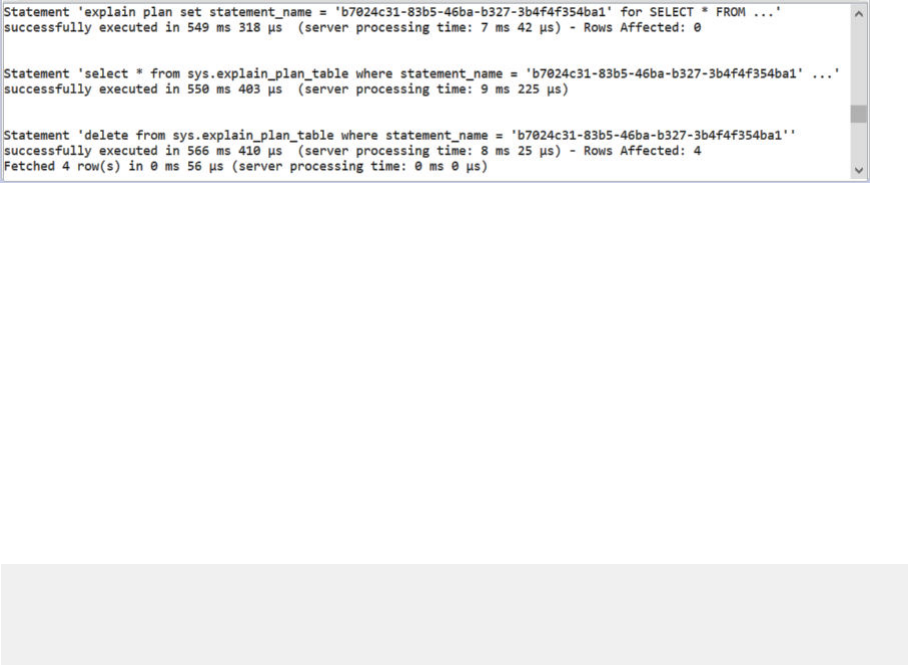
An example is shown below:
Since these processes are all done at once, there is no room for intervention. You cannot revisit the Explain Plan
that you have just created because it has already been deleted from the table. To revisit it, you need to recreate
it. In this context, it is more useful to extract the Explain Plan using the SQL plan cache because the caches are
always stored for later use (unless evicted), and therefore so are their plans.
Using the SQL Plan Cache and Plan ID
The best way to obtain the Explain Plan is to use the SQL plan cache, which has a consistent state and ensures
that the Explain Plans of the currently cached plans are also available.
You can use SQL statements like the following to obtain the Explain Plan from the SQL plan cache:
SELECT "PLAN_ID"
FROM "M_SQL_PLAN_CACHE"
WHERE "STATEMENT_STRING" LIKE '%<part of the SQL statement string>%';
EXPLAIN PLAN FOR SQL PLAN CACHE ENTRY '<plan ID>';
Using the SQL plan cache, you can always revisit the Explain Plan based on its plan ID. This also makes
performance troubleshooting possible and easier.
Often in performance tuning projects and performance consulting, the issue cannot be reproduced. A
performance issue experienced at a customer site long ago no longer occurs even when the same query is
executed at the same site in the same manner by the same user. Also, if a trace no longer exists, the issue can
no longer be tracked.
In contrast, users generally expect the system to capture every single plan that has been executed so they can
revisit any of these plans later. To that extent, Explain Plan is the one and only trace where the displayed tabular
plan is the one that was compiled in the early phase of the issue, because it pulls the plan directly from the SQL
plan cache using the plan ID.
Note that even the Plan Visualizer requires the exact SQL statement to utilize the cache and matching that
statement with the exact cache entry you want is not always easy. The Explain Plan is therefore recommended
as the rst performance tuning strategy for developers and performance tuning experts.
Related Information
Analyzing the Explain Plan [page 56]
Explain Plan Characteristics [page 59]
SAP HANA Performance Guide for Developers
SQL Query Performance
P U B L I C 55
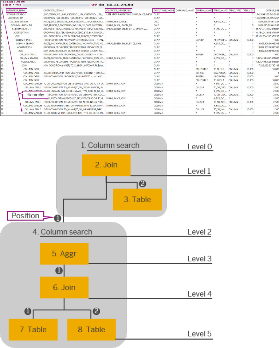
5.3.2.1 Analyzing the Explain Plan
This example shows how to read and interpret the information shown in the Explain Plan.
An Explain Plan is shown in the example below:
The Explain Plan is read through the hierarchy as follows:
56
P U B L I C
SAP HANA Performance Guide for Developers
SQL Query Performance
Using the OPERATOR_ID, PARENT_OPERATOR_ID, LEVEL, and POSITION, you can infer the location and the
level of the operator within the tabular plan. As seen from the example, the operator has a unique ID given to
each node. The nodes can be located using their parent operator ID. For example, the second column search
(4) from the top is the child of its parent Join (2) and parent of its child Aggregation (5). Along with this parent-
child hierarchy, the Explain Plan also oers a level-based hierarchy by simply displaying the level on which each
node resides. For example, the column search (4) is on the same level as the table (3), that is, on level 2, where
the former is the rst child and the latter the second child, and their positions are indicated by 1 and 2
respectively. Using these two types of hierarchies, the entire Explain Plan table can be restored even when its
original order has been broken. Normally, there is no need to use the hierarchy information because the
hierarchy can be easily identied through the indentation.
Operator Information
OPERATOR_NAME, OPERATOR_DETAILS, and OPERATOR_PROPERTIES provide information about the
operators. There are many operator names, ranging from the simple JOIN, FILTER, and LIMIT to SAP HANA-
specic operators like COLUMN SEARCH, ROW SEARCH, and MATERIALIZED UNION ALL.
Some of the operator names, such as FILTER and LIMIT, are not engine-specic, so you need the
EXECUTION_ENGINE information to know if it is a column engine operation or a row engine operation.
Together with the operator name, operator details provide useful information such as lter conditions, join
conditions, the aggregation type, grouping columns, partition information, and so on. They are usually human
readable and recognizable, so you can always consult this column to check whether there was an unwanted
grouping column during an aggregation operation, if a complex calculation was done simultaneously with other
operations like an aggregation or join, or if redundant columns were pulled for projection.
Size and Cost Information
Information about the estimated size and cost is provided in the columns TABLE_SIZE, OUTPUT_SIZE, and
SUBTREE_COST.
Table size is the estimated number of rows in the base tables. It does not show estimations for any of the
operators but only for the tables that are directly accessed, for example, physical column-store tables and
physical row-store tables. Although this is simply a table size, it is one of the gures which you can easily obtain
using the SQL console and which can sometimes help you nd a root cause. In rare cases, when the table size
estimation is incorrect, it can make the entire size and cost estimation of the plan wrong. Therefore, this
column is worth checking particularly when a thorough analysis has not helped you nd the root cause of a
performance degradation. Also, if the tables are too small or too big or if they do not have any data at all, there
is a higher risk of incorrect table size estimations, which may therefore need your attention if there is a
performance issue.
SAP HANA Performance Guide for Developers
SQL Query Performance
P U B L I C 57
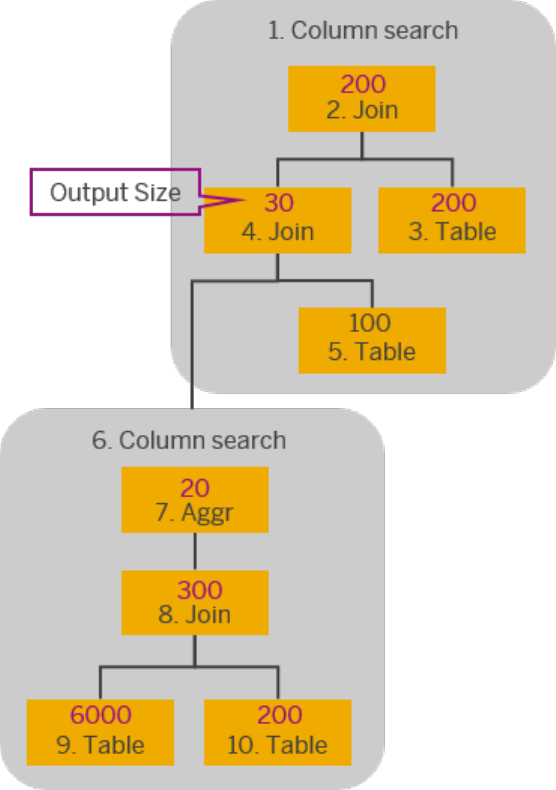
Output size is the estimated output size of each operator. For example, if the output size of the rst join from
the top with the operator ID 2 is 30, this means it will generate 30 rows if you selected the data right after that
join. In other words, the intermediate result of this subtree equals 30, as shown below:
Whenever you address any kind of performance issue, you focus on the operators, levels, engines, and anything
with a large or comparatively large size. In the Explain Plan, you can easily spot the level with a large estimated
output size, which is then a starting point for analyzing the performance issue.
Subtree cost is the calculated cost of the subtree. Basically, cost is a product of arithmetic calculation using
size as its core variable. Subtree cost is the same. Since subtree cost is to some extent proportional to subtree
size, as already seen above, the bigger the subtree size, the larger the cost. It is hard to decide what unit of
measure to use with the given cost values because the gure is relative rather than absolute. A large subtree
cost is a relative measure of the time needed to execute a subtree. The nal goal of your performance tuning
should therefore be to minimize the subtree cost.
58
P U B L I C
SAP HANA Performance Guide for Developers
SQL Query Performance
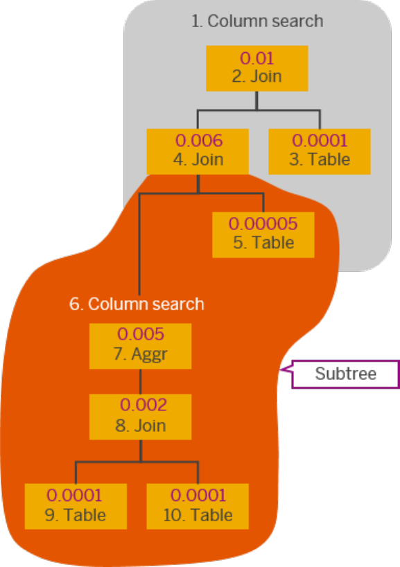
A subtree is shown in the example below:
5.3.2.2 Explain Plan Characteristics
The Explain Plan is a fast lightweight tool that provides a trace in tabular form.
Fast and Lightweight
One of the main advantages of using the Explain Plan is that it does not require the query to be executed. This
is what makes the Explain Plan useful when it comes to hard-to-reproduce issues like out of memory, system
hang, and system crash. These types of issue should not be reproduced, or if they need to be, this must be
done with great care, because reproducing them obviously means causing identical system failures. Therefore,
as a performance consultant, performance tuning expert, or developer, you should not run the SQL statement
SAP HANA Performance Guide for Developers
SQL Query Performance
P U B L I C 59
at issue particularly when it is on a production system. In those circumstance, the Explain Plan is very useful
because the query only needs to be compiled.
Tabular Data
A tabular form makes it easier to understand, compare, and analyze information. Since the Explain Plan is the
one and only trace that is in tabular form, it can be of great use when summarized information is needed. The
Explain Plan is particularly good for analyzing small-sized plans, because the whole table can t onto the
screen. You can easily recognize the levels through the indentation, see patterns, and follow gures to nd the
hot spot.
Repeated Engine Usage Pattern
It is sometimes easier to see execution engine patterns with the Explain Plan than with the Plan Visualizer, even
though the Plan Visualizer is unquestionably easier to follow due to its visualized format. However, when more
than three engines are involved in one plan, the shape of the tree cannot be clearly seen in the Plan Visualizer.
Although this is not often the case, the pattern of execution engine changes available in the Explain Plan is
sometimes better than in the Plan Visualizer.
5.3.3 Plan Visualizer
The Plan Visualizer (PlanViz) is used to create a visualized plan. A visualized plan is a visual map of the
operators and their relationships and hierarchies, which are described in a large single tree.
Although the Plan Visualizer seems simple because it merely makes existing information visual, the Plan
Visualizer is a powerful tool that you need to use multiple times throughout your entire analysis, at the
beginning to nd a hot spot, in the middle to get more ideas and information, and at the end to conrm your
ndings.
The Plan Visualizer is intuitive but also complicated and comprehensive at the same time. This means that it
can be both a starter and an enhancer depending on your context, the level of analysis you are applying, the
information you are looking for, and how deeply involved you are with the Plan Visualizer.
Single Statement Tracing
Like the Explain Plan, the Plan Visualizer is a feature of the SAP HANA studio. You can use the Plan Visualizer by
selecting the statement you want to trace and choosing Visualize Plan in the context menu.
Oered as a sub-option, the trace can be done after execution or just after preparation. The Executed Plan
provides actual information and not only planned information. Actual information can include the actual sizes
of the used operators, the inclusive/exclusive execution time for each level, the execution timeline, network
information, thread information, and so on. In contrast, the Prepared Plan only shows the data that is available
60
P U B L I C
SAP HANA Performance Guide for Developers
SQL Query Performance
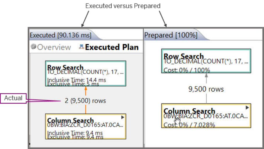
before the execution, such as the estimated size. Compared to the Executed Plan, the Prepared Plan is
lightweight but lacking in the information it provides. Most of the time, you will nd the Executed Plan more
useful.
An Executed Plan and Prepared Plan are shown in the example below:
The statements that you can trace with the Executed Plan include procedure calls as well as plain SELECT
statements. In the case of procedure calls, there are multiple visualized plans for the individual SELECT
statements within the procedure. The number of statements and how they are formatted depend on how the
procedure is inlined.
Time-based Multiple Statement Tracing
The Plan Trace is another way of tracing SQL queries and their execution plans. For example, if you go to the
trace section of the Administration editor in the SAP HANA studio, the Plan Trace is on the bottom right.
The Plan Trace creates a visualized plan for all statements that are executed during the trace time. The scope of
the trace is not conned to a single statement. Therefore, it is only useful when you want to make sure that
every statement is executed.
A case in point is when one of the clients running multiple statements on the database has a performance issue
but it is not certain which of those statements is causing the issue. However, other traces such as the debug
traces can also be used in these circumstances. In fact, the debug traces are recommended over the Plan Trace
because the Plan Trace has a very high memory usage. If you need traces for all SQL statements that are
executed during a certain timeslot, you should therefore opt for lighter traces like the debug traces unless the
visualization is critical for your analysis.
SAP HANA Performance Guide for Developers
SQL Query Performance
P U B L I C 61
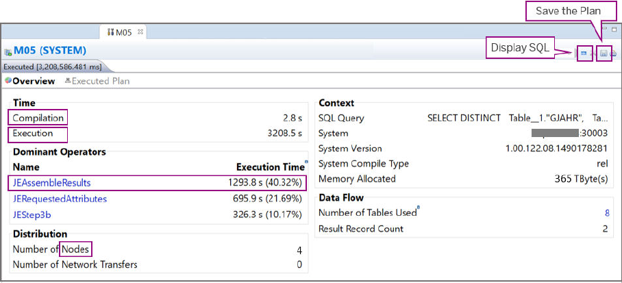
Related Information
Plan Visualizer Overview [page 62]
Node Information [page 63]
Logical versus Physical Executed Plan [page 63]
Actual versus Estimated Size [page 65]
Timeline, Operator List, Tables Used, Performance Trace, Network [page 66]
Plan Visualizer Characteristics [page 67]
NO_INLINE and INLINE Hints
5.3.3.1 Plan Visualizer Overview
After executing the Plan Visualizer or opening a Plan Visualizer le on the disk, the initial page you see is the
Overview. It contains all kinds of information, including most importantly the compilation time, execution time,
dominant operators, node distribution, SQL statement, and possibly system version.
An Overview is shown in the example below:
The time KPIs tell you how much time was consumed. The execution time indicates the signicance of an issue.
If the execution time is 2 seconds, it is not very critical even if users complain that the query is slow. But if it
takes 3,000 seconds to run a single SQL statement, this can be very critical because users need to wait 50
minutes for a result. Of course, how critical an issue is also depends on the business use case and
requirements. But from a developer's perspective, execution time can be regarded as a standard for
understanding how important an issue is.
Another factor to consider is the compilation time. Just because a query seems to be running slowly, it does
not mean that the performance issue has been caused by slow execution. Around 20 percent of these issues
are caused by slow compilation. Therefore, you should always consider the compilation time as well,
particularly when the execution time is not as high as reported. It is highly likely that this dierence is due to the
compilation time.
62
P U B L I C
SAP HANA Performance Guide for Developers
SQL Query Performance
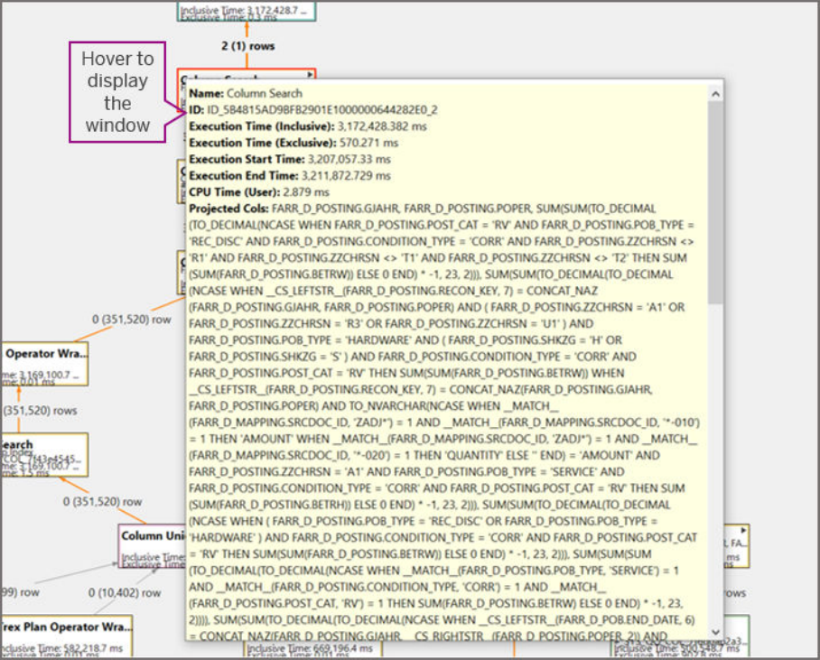
5.3.3.2 Node Information
One of the simplest ways to nd hidden information in the Plan Visualizer is to just hover your mouse over any
of the displayed nodes.
This method is particularly useful for getting information about join conditions, lter conditions, calculated
column information, expressions, projected columns, and even intermediate result names, and so on. However,
you should note that the displayed window disappears as you move your mouse around, so you may want to
paste the information to a text editor to have a better look at it.
Hover to display more information, as shown in the example below:
5.3.3.3 Logical versus Physical Executed Plan
The logical plan gives you the big picture and an overview of the plan, but it does not provide detailed
information such as execution engine information. Physical plans contain more detailed information, including
information which is provided by the execution engines. Physical plans are usually complex.
The logical plan shows the shape of the query optimizer (QO) tree and contains structural information. Before
analyzing the physical plan, you should rst analyze the logical plan. Having found some starting points and
SAP HANA Performance Guide for Developers
SQL Query Performance
P U B L I C 63
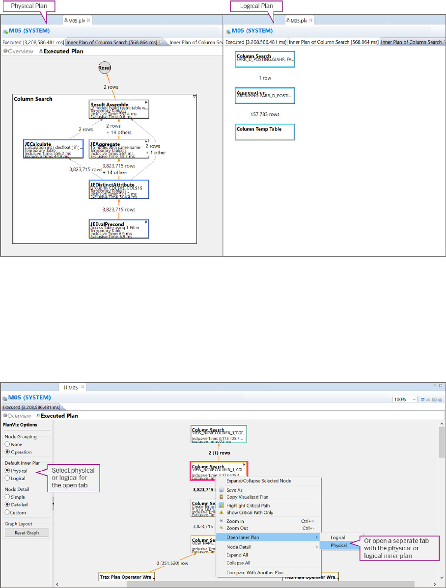
possibly a hot spot, you can proceed to the physical plan. Generally, your analysis should be performed from
the logical plan to the physical plan and not the other way around.
A logical plan and physical plan are shown in the example below:
Note that when analyzing a physical or logical plan, you don’t have to move an entire plan from physical to
logical or vice versa just to view certain information. In the physical plan, column searches are folded by default
into a single node to ensure a tidy display. If you want to keep your physical plan clean or keep the logical plan
but still see a physical plan of one of the logical nodes, you can open a separate tab to display the additional
information. To do so, select the node and from the context menu choose Open Inner Plan.
The example below shows how you can open a physical or logical inner plan. It can either be selected as the
default type for the open tab under Default Inner Plan, or an additional tab can be opened with the physical or
logical inner plan by using the context menu:
64
P U B L I C
SAP HANA Performance Guide for Developers
SQL Query Performance
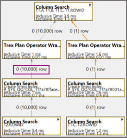
5.3.3.4 Actual versus Estimated Size
To understand the behavior of the SQL optimizer, it is very helpful to compare the actual value to the estimated
value.
In the Executed Plan, there are two gures for data size. The gure in parentheses is the size estimated by the
optimizer and used during query compilation. The gure without parentheses is the actual gure, which is only
available after execution. Since the optimization process of a query depends heavily on cost estimation, and
therefore also on size estimation, a large dierence between the two gures is signicant because it indicates
that the optimizer's work did not have a solid basis. Optimization is essentially an assumption, despite its
scientic, algorithmic, and mathematic traits. Assumptions can therefore only perform well when they have a
solid basis. When a large dierence is seen between the actual and estimated sizes, the inaccuracy of the
estimated size is a potential cause of the performance issue. A large dierence generally means a dierence of
over a million. Smaller dierences could have a small impact and sometimes no impact at all.
When the dierence is tracked down to the base table layer, it is sometimes found that the table size was
incorrectly estimated in the rst place. If this is the case, you need to check other traces like the Explain Plan
and possibly the debug traces to conrm your ndings. One of the cases could be that the estimated table size
is 10,000 whereas the table is in fact empty. This behavior is expected because when a table is empty the
optimizer considers its size to be 10,000. This means that your SAP HANA system is working correctly. In other
cases, more investigation is needed.
In the same way that empty tables can legitimately result in faulty size estimations, so can huge tables and
large operations. As intermediate results get bigger, an expected result is that the estimations are less precise.
If this is the case, one eective measure is to reduce the intermediate sizes by using lters or SQL hints.
The example below shows an empty table with an estimated size of zero:
Apart from the dierence in the gures discussed above, the size gure itself can also indicate the root cause of
the problem. For example, suppose an out-of-memory condition occurred that can be reproduced by executing
an SQL statement and its visualized plan is obtained. In the Plan Visualizer, you can easily see on which
operation the execution failed, unless the system did not have enough memory to even draw the visualized
plan. If the failure point is one of the join nodes and one of its children is very large, containing for example a
billion rows, this immediately gives you an idea why the operation failed. SAP HANA is an in-memory database,
SAP HANA Performance Guide for Developers
SQL Query Performance
P U B L I C 65
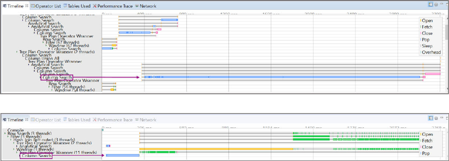
which requires that memory is used smartly and eciently. If so many records are to be operated on, it will run
out of memory. In this context, it is worth remembering that the maximum number of records allowed in a
single table in SAP HANA is 2 billion, and temporary tables are not an exception. So, if the failed join in this case
were to be materialized, the execution would have failed anyway.
The actual and estimated sizes are therefore important. It is highly recommended that you keep an eye on the
sizes whenever you start analyzing a performance issue.
5.3.3.5 Timeline, Operator List, Tables Used, Performance
Trace, Network
Although it depends on how you organize your display, the panels in SAP HANA studio that contain more
detailed information are by default located at the bottom. When you examine the visualized plan in the main
window, it is easy to overlook these additional windows, which also provide important information.
The Timeline view provides detailed information about the duration of each operation, for example, the
duration of a fetch or pop operation for a single column search. The parallel thread information is generally
more important as well as any dominant time-consuming thread. In the main window of the visualized plan, you
cannot infer which of those operations were started or executed at the same time, and which operation ended
before the other. However, in the
Timeline view, which shows all operations on a timeline, the parallel executions
are explicitly displayed with their starting points and completion points.
The Timeline view is also useful is when there is a dominant thread that cannot be explained. On the Overview
tab, it is simple to pinpoint the dominant operator by clicking Dominant Operators. In the Timeline view,
however, you can analyze whether the performance lag is the result of a slow pop operation or other slow
processes, like a slow fetch operation or slow compilation. If it proves to be a slow pop operation, you can safely
start analyzing the plan and tackling the hot spot. If the slowness is caused by non-reducible factors like
opening, fetching and closing, this is outside the scope of your analysis. If it concerns compilation, like ce-qo
(calculation engine query optimization) compilation, you need to investigate it further using various debug
traces.
In the example below, the rst column search that is outlined is problematic, the second is not:
The Operator List, Tables Used, and Performance Trace are useful when you want to search for a text or order
the operators because they are in a tabular form. For example, when the plan is complex and you want to focus
on a specic lter or expression, you can search for the terms here. It is also possible to order the operators by
66
P U B L I C
SAP HANA Performance Guide for Developers
SQL Query Performance
their exclusive execution times in descending order so that you can compare the durations between the
operators.
The Network view allows you to check the network packages transmitted between the dierent nodes. This is
sometimes very useful and even decisive for root-cause analysis, particularly when there is a network issue and
the Network view shows abnormal package transfers. When multiple nodes are involved, it worth checking the
Network view.
5.3.3.6 Plan Visualizer Characteristics
Since the Plan Visualizer is almost the only way you can see a query plan in a visualized manner, it is a very
good tool to start with.
Visualized Tree
By zooming out of the tree, the overview can give you an idea of the query's complexity, volume, repeated tree
patterns, and repeated operators. This is particularly advantageous when there are two or more traces that you
want to compare, for example, when you have a plan that runs slowly and another plan with the identical query
that runs faster. To nd the dierence between the two, you can open both visualized plans side by side and
compare the zoomed-out trees.
A visualized plan is a huge le that contains complex information, although it might seem like all this
information is hidden because it is distributed in several locations like bottom panels, hover boxes, and side
windows. The Plan Visualizer is therefore both a starting point and a nishing point. It gives you both a broad
(macroscopic) and a detailed (microscopic) view of the same plan at the same time.
Actual Size of Executed Operators
Actual execution information is only available in the Plan Visualizer. It is not provided by the Explain Plan. Actual
sizes are shown without parentheses, whereas planned gures are shown within parentheses. A large
dierence between the two gures can be signicant.
Note that the actual size shown in the Plan Visualizer is not always applicable to every case you have. That is
because this trace is only available after the plan has been executed. Let's say there is a query raising an out of
memory (OOM), but you don't have any traces. Although you know that the Plan Visualizer could help your
analysis considerably, you cannot create this trace because the system would run out of memory again. This
situation is even worse when the case concerns a system crash. In the OOM case, you would get a visualized
plan at the cost of an OOM. In the case of a system crash, your only option is to use the Explain Plan to analyze
the plan because it doesn't require the query to be executed. Therefore, you need to be aware of the pros and
cons of the Plan Visualizer and Explain Plan so that you can apply the correct one when needed.
SAP HANA Performance Guide for Developers
SQL Query Performance
P U B L I C 67

5.3.4 SQL Trace
The SQL trace captures every single SQL statement that enter the database. It works on the session layer.
If you cannot nd an SQL statement in this trace, there are two possible reasons. Either the statement was
never executed in this database, or the statement never reached the session layer because it was executed
internally, in which case it would not have had the form of an SQL statement anyway. One exception is where a
statement is propagated internally and transmitted back to the session layer in the form of an SQL statement.
This statement is not captured by the default SQL trace setting. However, this internal statement can be logged
when you enable the "internal statement" conguration setting, as described below.
Single Statement Tracing
The SQL trace can be congured in two ways. One way is on the Trace Conguration tab of the Administration
editor in the SAP HANA studio. You can do the same thing by simply running an SQL statement in the SQL
console.
Enabling the Trace with SAP HANA Studio
The SQL trace is on the top right of the Trace Conguration tab of the Administration editor in the SAP HANA
studio. To activate the trace, you need to click the pencil icon and enter the appropriate context information. It
is recommended that you use as many lters as possible, because otherwise the script will be very long. It is
important to use script-based traces eciently because it can take a very long time to download a script, just
to nd a single line of the SQL statement that you are interested in. This applies not only to the SQL trace but to
all other kinds of congurable or script-based traces as well, such as the SQL Optimization Step Trace.
To turn o the SQL trace, you need to click the same pencil icon again and then set the trace to inactive. You
can nd the trace le on the Diagnosis Files tab of the Administration editor.
Enabling the Trace with SQL
You can enable and disable the SQL trace by running the appropriate SQL statements in the SQL console. The
SQL statements for setting system conguration in SAP HANA start with ALTER SYSTEM. This is also the case
for the SQL trace conguration. The ALTER SYSTEM statement is used more frequently than the
Administration UI because it is always available, even without the SAP HANA studio interface, and is therefore
very convenient to use.
You can enable the SQL trace with the following SQL statement:
ALTER SYSTEM ALTER CONFIGURATION ('indexserver.ini','SYSTEM')
SET ('sqltrace','trace') = 'on',
('sqltrace','user') = '<database_user>',
('sqltrace','application_user') = '<application_user>'
WITH RECONFIGURE;
You can disable the SQL trace with the following SQL statement:
ALTER SYSTEM ALTER CONFIGURATION ('indexserver.ini', 'System')
UNSET ('sqltrace', 'trace'), ('sqltrace','user'),
('sqltrace','application_user') WITH RECONFIGURE;
68
P U B L I C
SAP HANA Performance Guide for Developers
SQL Query Performance

Multiple Statements from a Procedure Call
Some SQL statements are initiated internally and then sent all the way back to the session layer. The
representative case in point is when a procedure is run. Although a procedure is a collection of multiple SQL
statements, the statements contained in the denition are not executed individually.
When compiling the procedure, the SQLScript optimizer combines two or more of the statements if their
combined form is considered to be more ecient. This process is called inlining and is usually benecial for
most procedures. Unless congured otherwise or prevented through hints, a procedure is inlined, so you never
know what SQL statements the procedure was divided into. However, when the SQL trace has the "internal
statement" option activated, you can nd this out. Because the SQL statements spawned from the procedure
are built and executed internally, they are only captured if the SQL trace is explicitly congured to include
internal statements. To do so, the internal option needs to be enabled (set to true) for the SQL trace. When
this option is enabled, the internal statements are also recorded in the SQL trace. If the query_plan_trace is also
enabled and the level option set appropriately, the trace will also include each statement's plan explanation as
well as its records, which are shown in arrays.
You can enable the internal SQL trace with the following SQL statement:
ALTER SYSTEM ALTER CONFIGURATION ('indexserver.ini','SYSTEM')
SET ('sqltrace','trace') = 'on',
('sqltrace','user') = '<database_user>',
('sqltrace','application_user') = '<application_user>',
('sqltrace','query_plan_trace') = 'on',
('sqltrace','internal') = 'true',
('sqltrace', 'level') = 'all_with_results'
WITH RECONFIGURE;
You can disable the internal SQL trace with the following SQL statement:
ALTER SYSTEM ALTER CONFIGURATION ('indexserver.ini', 'System')
UNSET ('sqltrace', 'trace'), ('sqltrace','user'),
('sqltrace','application_user'), ('sqltrace','internal'),
('sqltrace','query_plan_trace'), ('sqltrace', 'level')
WITH RECONFIGURE;
Related Information
Analyzing the SQL Trace [page 69]
5.3.4.1 Analyzing the SQL Trace
The purpose of SQL trace is to nd the statement at issue. The problem is that it is often not that easy to nd it
in the log stack.
The following example shows an SQL statement and the context information that can help you nd it:
SAP HANA Performance Guide for Developers
SQL Query Performance
P U B L I C 69
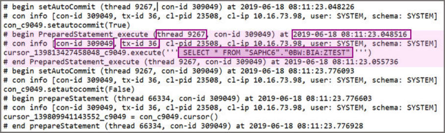
It is important to know the time frame during which the statement ran. The narrower it is, the easier it will be. If
you don't know the thread number or the transaction ID associated with the statement, you should look for the
schema name. In the editor where the trace le is open, search for the name of the schema containing the
business data, for example, "/SAPPRD" in the Vim editor. There might be several statements that were
executed during the specic time frame using the tables in the specied schema. You should also see other
information such as the thread and transaction ID.
The SQL trace can also be used in reverse, for example, to nd the precise timestamp of the statement
execution. There can also be cases where you already know the thread number and you want to track down the
execution time or the statement string. By juggling these key pieces of information, you should be able to nd
the details you are looking for.
5.3.5 SQL Optimization Step Debug Trace
The SQL optimization step debug trace (also referred to as the SqlOptStep trace) logs the shape and contents
of the query optimization (QO) tree captured in each step of the optimization.
As described in the SQL optimizer topics, there are two main categories of optimization, rule-based rewriting
and cost-based enumeration. In the case of rule-based rewriting, the SQL optimization step trace shows what
the QO tree looks like after each rule has been applied. For example, you can see that the QO trees before and
after calculation view unfolding are dierent. In the case of cost-based enumeration, the SQL optimization step
trace shows the logical tree and the physical tree of the nal execution plan. While the logical execution plan
indicates which operators are located where, the physical execution plan tells you which types of operators
were selected.
The SQL optimization step trace also provides more detailed information at the debug level. This includes
estimated sizes, estimated subtree costs, applied rule names, applied enumerator names, partition
information, column IDs, relation IDs, and much more.
The fastest and most eective way to learn about the SQL optimization step trace is to use it yourself. This
means working through all the activities required to collect the trace and analyze it.
70
P U B L I C
SAP HANA Performance Guide for Developers
SQL Query Performance
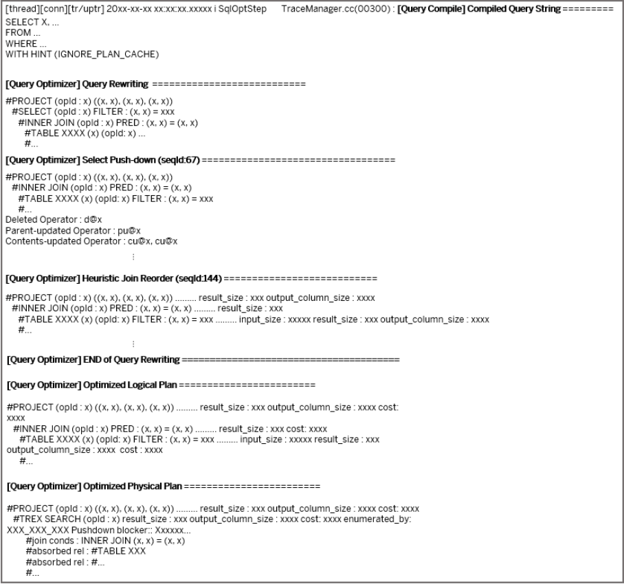
The example below shows the format of the SQL optimization step trace:
Collecting the SQL Optimization Step Trace
The SQL optimization step trace logs the optimization steps applied by the SQL optimizer and can therefore be
used to investigate the optimizer's behavior during the optimization phase. The trace should therefore only be
collected during query compilation.
It is important to ensure that the query undergoes the compile phase because otherwise the SQL optimization
step trace will be empty. If the query is not compiled, it results in a cache hit, the SQL optimizer is omitted, and
the executors use the cached plan.
There are two ways to obtain an SQL optimization step trace when a cache already exists. You can either delete
the cache or force the query to skip the cache hit. For information about how to delete the SQL plan cache, see
the SQL plan cache Maintenance topic. You can force the query to skip the cache by using the hint
SAP HANA Performance Guide for Developers
SQL Query Performance
P U B L I C 71

IGNORE_PLAN_CACHE. This prevents the query execution from reading from and writing to the SQL plan
cache.
Related Information
Maintenance [page 54]
Enabling the SQL Optimization Step Trace with SQL [page 72]
Using Tags for Easier Analysis [page 73]
Extra Filters for a More Ecient Trace [page 73]
Session Debug Trace [page 74]
Analyzing the SQL Optimization Step Trace [page 74]
Optimized Logical and Physical Plans [page 76]
5.3.5.1 Enabling the SQL Optimization Step Trace with SQL
The most basic way to enable and disable the SQL optimization step trace is to use the ALTER SYSTEM
statement and set the parameter('trace', 'sqloptstep').
This trace will then be included in the index server trace, which is the database trace that, by default, is always
on in order to log every activity that occurs on the index server on the INFO level. By enabling the additional
trace, you are in eect raising the severity level of the index server trace for this specic component. To make
your investigation more ecient, you might want to add a user lter by setting the sql_user parameter to the
database user ID. This should give you a shorter but more productive result.
But in most cases, you need a separate trace le rather than an index server trace that contains the SQL
optimization step trace together with all kinds of other INFO traces. The "traceprole" conguration enables
you to customize the name of the le to which the trace will be written. For example, by setting the
conguration to traceprofile_MyTrace01, a le named
indexserver_<hostname>.<port>_MyTrace01.trc will be written which only contains the SQL
optimization step trace.
Although the simple way of enabling the trace with ('trace', 'sqloptstep') has been mentioned here,
this is only to give you an idea of how this trace works. For most use cases, the more practical and preferred
method is to use ('traceprofile_<keywords>', 'sqloptstep'), which provides the information that
you really want. In many cases, you can use this parameter to indicate the purpose of the trace. For example,
you could try using keywords like ('traceprofile_20190620_17sec', 'sqloptstep') or
('traceprofile_SqlOptStep_GoodCase', 'sqloptstep'). These labels will help you to easily spot the
le you need in the list.
You can enable and disable the internal SQL optimization step trace with the following SQL statements:
● Basic method:
ALTER SYSTEM ALTER CONFIGURATION ('indexserver.ini','SYSTEM')
SET ('trace','sql_user') = '<database_user>',
('trace','sqloptstep') = 'debug'
WITH RECONFIGURE;
ALTER SYSTEM ALTER CONFIGURATION ('indexserver.ini','SYSTEM')
72
P U B L I C
SAP HANA Performance Guide for Developers
SQL Query Performance

UNSET ('trace','sql_user'), ('trace','sqloptstep')
WITH RECONFIGURE;
● Advanced method:
ALTER SYSTEM ALTER CONFIGURATION ('indexserver.ini','SYSTEM')
SET ('traceprofile_MyTrace01','sql_user') = '<database_user>',
('traceprofile_MyTrace01','sqloptstep') = 'debug'
WITH RECONFIGURE;
ALTER SYSTEM ALTER CONFIGURATION ('indexserver.ini','SYSTEM')
UNSET ('traceprofile_MyTrace01','sql_user'),
('traceprofile_MyTrace01','sqloptstep')
WITH RECONFIGURE;
5.3.5.2 Using Tags for Easier Analysis
When you start any type of trace, you should know how you intend to analyze it. To make the analysis easier, it
helps to add tags in the executed statement.
For example, you could add /*literal*/ and /*parameterized*/ if you want to compare a literal query
with a parameterized query. Or you could use /*Good_17_seconds*/ and /*Bad_300_seconds*/ if you
intend to compare plans with dierent levels of performance.
The SQL optimization step trace nearly always involves comparison. Therefore, it is important to make each le
or trace unique so that it can be easily recognized, and you and other users do not confuse it with another one.
5.3.5.3 Extra Filters for a More Ecient Trace
If you have the SQL user lter and trace le name congurations in place but still get noise from other queries
executed by the same user, you need more meticulous lters to remove that noise. The statement hash and
connection ID are the two main lters you can use.
You can add extra lters to the SQL optimization step trace with the following SQL statement:
ALTER SYSTEM ALTER CONFIGURATION ('indexserver.ini','SYSTEM')
SET ('traceprofile_MyTrace01','sql_user') = '<database_user>',
('traceprofile_MyTrace01','sqloptstep') = 'debug',
('traceprofile_MyTrace01','statement_hash') = '<stmt_hash>',
('traceprofile_MyTrace01','connection_id') = '<connection_id>'
WITH RECONFIGURE;
You can remove the extra lters from the SQL optimization step trace with the following SQL statement:
ALTER SYSTEM ALTER CONFIGURATION ('indexserver.ini','SYSTEM')
UNSET ('traceprofile_MyTrace01','sql_user'),
('traceprofile_MyTrace01','sqloptstep'),
('traceprofile_MyTrace01','statement_hash'),
('traceprofile_MyTrace01','connection_id')
WITH RECONFIGURE;
SAP HANA Performance Guide for Developers
SQL Query Performance
P U B L I C 73
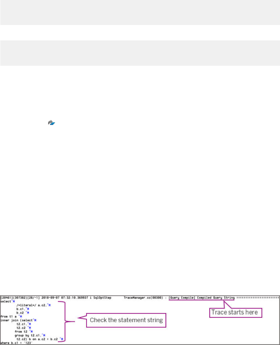
5.3.5.4 Session Debug Trace
You can use a separate session and trace only that session for the component you are interested in. For more
information, see SAP Note 2380176.
You can set a session for the SQL optimization step trace with the following SQL statement:
ALTER SYSTEM ALTER CONFIGURATION ('indexserver.ini','SYSTEM')
SET ('traceprofile_MyTrace01','sqloptstep') = 'debug' WITH RECONFIGURE;
SET SESSION 'TRACEPROFILE' = 'MyTrace01';
You can remove a session for the SQL optimization step trace with the following SQL statement:
UNSET SESSION 'TRACEPROFILE';
ALTER SYSTEM ALTER CONFIGURATION ('indexserver.ini','SYSTEM')
UNSET ('traceprofile_MyTrace01','sqloptstep') WITH RECONFIGURE;
Related Information
SAP Note 2380176
5.3.5.5 Analyzing the SQL Optimization Step Trace
Compiled Query String
To be able to analyze trace information eciently, it is important to know on which line of the trace le the trace
you requested starts.
To nd the starting point, you need to look for Compiled Query String. The information it provides is not that
helpful because it simply tells you the thread, connection ID, transaction ID, and timestamp. However, it
represents the starting line of the trace and is therefore the point at which you should start your analysis.
For example:
74
P U B L I C
SAP HANA Performance Guide for Developers
SQL Query Performance
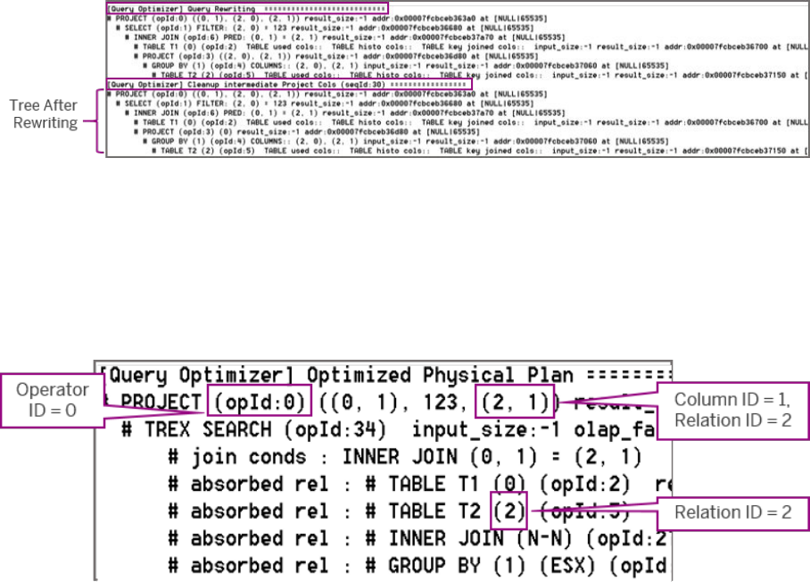
Query Rewriting
This section has the prex Query Optimizer contained within square brackets. The SQL optimization step trace
lists the names of the query rewriting rules and species the QO tree directly after each step of rewriting. For
example, under [Query Optimizer] Select Push-down (SeqId:nn), you would see the QO tree after the rule
Pushdown has been applied to the tree. This pattern is repeated until query rewriting reaches the cost-based
optimization step.
An example of a [Query Optimizer] Query Rewriting section is shown below:
QO Tree Component Basics
The components that form the QO trees under the rewriting rules are also important for the analysis.
For example:
The overall shape of the tree is very similar to the Explain Plan. Indentation is used to represent the hierarchy,
that is, the more a line is indented, the lower it is in the hierarchy. Each line starts with a hash character (#),
which is followed by the name of the operator, such as PROJECT, INNER JOIN, or TABLE, with its ID number at
the end in the form (opId : nn). The opId is simply a unique ID given to each operator and used by the
optimizer to manage them. These IDs can also be used for plan analysis because they are unique and therefore
make the operators easy to identify. For example, if you want to track every change made to a specic operator,
you just need to track its operator ID. To help with this procedure, there are additional lines that indicate all
changes that were made to the operators. These are shown at the bottom of each QO tree after the rewriting
names using the categories Deleted Operator, Parent-updated Operator, and Contents-updated
Operator. The number d@ after the Deleted Operator: is the ID of that deleted operator. Similarly, the
numbers after pu@ and cu@ indicate those operators where either their parents' or their own content has been
updated.
An understanding of the basic concepts of relation IDs and column IDs is needed for trace analysis. A relation is
a logical data set produced or consumed during an operation. For example, a table is a relation and an
SAP HANA Performance Guide for Developers
SQL Query Performance
P U B L I C 75

aggregated set of the table is another relation. Each relation is given a unique ID, starting from the outermost
relation and moving inwards. Since a relation is a set of columns lled with data, each column is also given an
ID, starting from the leftmost column. A column in a relation is identied by two ID numbers in brackets with a
comma between them. For example, (4,1) denotes the second column from the left of the fth outer relation,
although it does not indicate what data it contains. To nd that information, you need to trace it back to the top,
possibly to table level, where you can see the name of the column.
Although it looks very complicated, it is important to understand and follow the relation IDs and column IDs
because very small changes in these IDs within a set of operations can make a huge dierence, even though
there might be no apparent reason. Sometimes one or two columns are dropped during one of the
aggregations, resulting in nal values that are unexpected. Other times there are just too many relations for the
same table, and you need to nd a way to combine them into one relation by deriving the appropriate lters or
removing joins.
On the surface of SQL, you see the names of tables and columns. Inside the optimizer, however, they are
distinguished by their IDs. Therefore, you need to familiarize yourself with these internal structures to be able
to analyze the internal operations of the optimizer.
Heuristic Rules
Heuristic rules are part of the rewriting rules, so the basic principles that apply to rewriting rules also applies to
heuristic rules. Heuristic rules, however, also show you the estimated sizes of the operators in the trace. This is
because heuristic rules themselves use estimated sizes.
Unless you specically need the sizes estimated by the heuristic rules in order to know where an estimation
was started, the estimated values are not a good tool for analysis because they are premature. If you intend to
analyze sizes and costs, it is better to do so using the values given in the Optimized Physical Plan.
For example, sizes are shown but can be ignored:
5.3.5.6 Optimized Logical and Physical Plans
Once rule-based query rewriting has nished, cost-based enumeration starts. The only information provided by
the SQL optimization step trace about cost-based enumeration is a few details about the logical and physical
aspects of the nal product. This is because you do not really need to know about all the processes that occur
during enumeration.
The enumeration trace does provide that information when it is enabled. However, the reason why the detailed
optimization processes were omitted from the SQL optimization step trace was to make it as compact as
possible. Therefore, it is not recommended to enable the enumeration trace unless a developer explicitly
advises you to do so.
Although they look simple and short, the two nal products of enumeration are very important and among the
most frequently used items in the entire trace. The Optimized Logical Plan resembles the logical subtree in the
76
P U B L I C
SAP HANA Performance Guide for Developers
SQL Query Performance
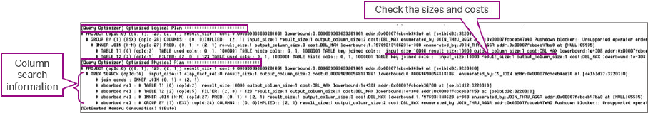
Plan Visualizer and Explain Plan, whereas the Optimized Physical Plan is like a physical subtree in the Plan
Visualizer and Performance Trace. While the Optimized Logical Plan shows the trunk and branches of the tree,
indicating the locations and logical shapes of the operators, the Optimized Physical Plan shows the types of
leaves the tree chose as well as execution engine-specic information and column search information.
For example:
In plan analysis, you usually start by searching for the tag that was commented out in the statement string in
order to nd the rst line of the trace. This takes you to the Compiled Query String line, where you can search
for the term Optimized Physical Plan to nd the plan details. You can then locate the Optimized Logical
Plan higher above, which is where you can start the actual analysis. The Optimized Logical and Physical Plans
should give you an impression of what the entire plan looks like and some information about why it was shaped
in this way.
5.3.6 SQL Optimization Time Debug Trace
The SQL optimization time trace (SqlOptTime trace) is a stopwatch that measures how much time it takes to
nish each step of the optimization.
It records not only the time required for the overall rule-based or cost-based optimization process, but it also
records the time consumed by each writing rule in rule-based optimization and the number of repeated
enumerators during cost-based optimization.
The stopwatch for the SQL optimization time trace starts when compilation begins and ends when it nishes.
The SQL optimization time trace is therefore primarily a compilation trace and not an execution trace. An SQL
optimization time trace can even be obtained by just compiling a query and cancelling it immediately before
execution. There is therefore no point in collecting this trace when you want to improve execution time,
particularly when the case involves an out of memory condition or long running thread caused by huge
materialization.
The SQL optimization time trace is helpful when there is a slow compilation issue. In relation to execution time,
there could be a case where a long execution time can only be reduced at the expense of a longer compilation
time, so the total time taken from compilation to execution remains the same irrespective of which one you
choose to reduce. In such cases, although it is an execution time-related performance issue, you still need the
SQL optimization time trace to investigate whether the compilation time could be improved. There could be
many other cases where a long execution time is closely related to compilation, such as the optimizer reaching
the enumeration limit, which causes it to stop and generate a plan. Or there might simply be a slow compilation
issue where the purpose of the investigation is to reduce the compilation time.
The SQL optimization time trace can also be used in a general sense just to get a summarized report of the
rules and enumerators used to make the nal plan. The SQL optimization step trace is usually very long and
you may therefore prefer a brief version that just tells you what choices the optimizer made rather than how
they were made. In that case, the SQL optimization time trace would be an appropriate tool.
SAP HANA Performance Guide for Developers
SQL Query Performance
P U B L I C 77
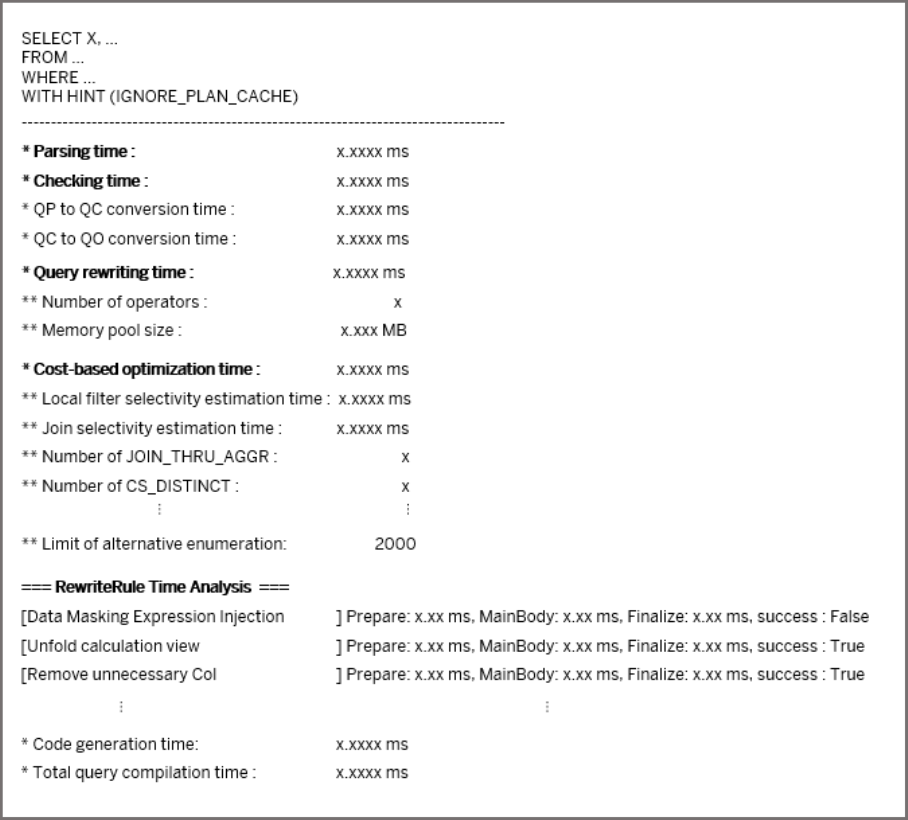

5.3.6.1 Enabling the SQL Optimization Time Trace
The SQL optimization time trace trace is as simple to use as the SQL optimization step trace. To enable the
trace, you just replace the conguration parameter sqloptstep with sqlopttime.
The only dierence between the traces is that the SQL optimization time trace starts logging when compilation
begins and ends at the point of execution. Even if you cancel the transaction, the SQL optimization time trace
will still be available, unless compilation was not completed.
You can enable the internal SQL optimization time trace trace with the following SQL statement:
ALTER SYSTEM ALTER CONFIGURATION ('indexserver.ini','SYSTEM')
SET ('traceprofile_MyTrace01','sql_user') = '<database_user>',
('traceprofile_MyTrace01','sqlopttime') = 'debug'
WITH RECONFIGURE;
You can disable the internal SQL optimization time trace trace with the following SQL statement:
ALTER SYSTEM ALTER CONFIGURATION ('indexserver.ini','SYSTEM')
UNSET ('traceprofile_MyTrace01','sql_user'),
('traceprofile_MyTrace01','sqlopttime')
WITH RECONFIGURE;
Note that because query compilation also occurs as part of calculation engine query optimization (CeQo) or
calculation engine SQL (CeSql) during execution, these compilation logs are also written in the trace. If you
therefore had CeQo in the plan, you would have two sets of SQL optimization time traces in one trace le at the
end.
This can be quite helpful for your analysis because CeQo compilation time is easily but incorrectly rendered as
execution when it is in fact compilation. There are cases where a long execution time is caused by a long CeQo
compilation time. The way to solve this problem would be to remove the CeQo by enforcing calculation view
unfolding or to make the view simpler by modifying the base calculation views.
5.3.6.2 Analyzing the SQL Optimization Time Trace
The SQL optimization time trace looks very dierent from other traces, so it is relatively easy to nd the trace
even when there are many lines in the index server trace.
The SQL optimization time trace has several dash lines and the content between the lines looks more like a
report than a log or trace. It lists the measured parameters with the values given in milliseconds (ms) or
megabytes (MB).
The SQL optimization time trace starts with the query string shown under [Query Compile] Compiled
Query String. It then lists the parsing time, checking time, query rewriting time, and cost-based optimization
time. In very rare cases, the parsing time or checking time could be unexpectedly long, say 10 seconds. This
would then need to be investigated further by the SAP HANA frontend experts. 99% of long compilation issues
involve either long query rewriting time or long cost-based optimization time.
SAP HANA Performance Guide for Developers
SQL Query Performance
P U B L I C 79
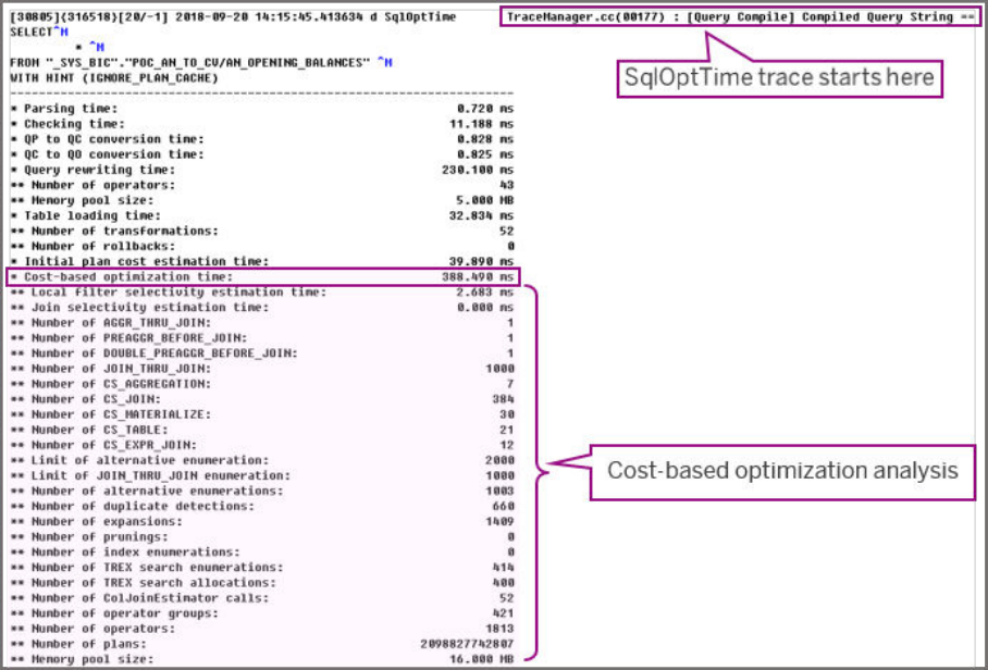
Cost-based Optimization Time Analysis
This analysis provides lter and join selectivity estimation times, the number of enumerations for each
enumerator, and the enumeration limit. The local lter selectivity estimation time is the time taken to calculate
the selectivity of the lters. The selectivity is a ratio of the values ltered out of the data set. For example, if the
values are very distinct and only one out of a hundred matches the lter condition, the selectivity would be
0.01.
But when the table or data source is too large for the entire set to be examined in a short time, SAP HANA
resorts to estimation strategies like sampling or histogram analysis. Almost all customer cases depend on
these estimation strategies, particularly sampling, where a maximum of 1,000 rows, by default, are collected as
a sample set and prorated into the whole. The local lter selectivity estimation time refers to the time required
for this process.
For example:
The join selectivity estimation time is the time required to calculate the join cardinality. The SQL optimization
step trace shows cardinality information like (N-N) or (N-1) next to the JOIN. The cardinality information
allows the execution time to be shortened because the rows that will eventually be dropped do not need to be
combined beforehand.
These estimation times are shown in the trace, but they rarely cause any problems because they are
mathematical calculations based on algorithms. Even so, if there are any problematic estimations, it is
advisable to provide this information to the SQL optimization experts at SAP.
The remaining information about cost-based optimization time consists of the number of enumerations of the
various types. For example, Number of JOIN_THRU_AGGR means how many times the enumerator
JOIN_THRU_AGGR (join through aggregation) was applied. If this number is too high, you may want to lower it
80
P U B L I C
SAP HANA Performance Guide for Developers
SQL Query Performance
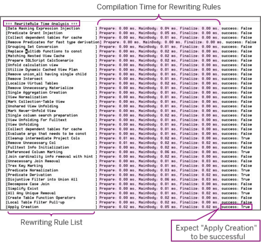
by using an SQL optimization hint. Let’s say JOIN_THRU_AGGR was done 1000 times. By adding the hint
NO_JOIN_THRU_AGGR, you can make the SQL optimizer choose not to push down the joins. This approach is
not an analysis strategy as such but it might help you get closer to your goal.
Rule-Based Optimization Time Analysis
A separate section called RewriteRule Time Analysis indicates whether each rewriting rule was processed
successfully and how long this took. Only the successful rewriting rules are relevant for you analysis, together
with the times (in milliseconds) given in all three sections, not just in Prepare or MainBody.
For example:
This section is helpful when one of the rules took too many milliseconds to complete. The most common
example is when the calculation view unfolding process takes too long. In this case, you should rst apply the
hint NO_CALC_VIEW_UNFOLDING so that this step is skipped. It is highly likely that the compilation time will
be reduced but at the cost of a longer execution time because the calculation engine may then take the CeQo
path instead. As seen before, there is a trade-o between the two major factors, compilation and execution. To
SAP HANA Performance Guide for Developers
SQL Query Performance
P U B L I C 81

nd a solution, you should consider how to remove the complex evaluation inside the calculation view that
requires so much time to be translated into a QO tree.
5.3.7 Views and Tables
Various views and tables are available for analyzing performance.
Expensive Statements
The expensive statements trace records information about a statement if its execution time exceeds the
specied threshold, which is 1 second by default. The contents of this trace are available in the monitoring view
M_EXPENSIVE_STATEMENT.S. The monitoring view collects the information from the disk les where the
records are stored. This means that once you have enabled the trace, you can simply download the
expensive_statements le from the SAP HANA trace directory or the Diagnosis Files tab of the SAP HANA
studio administration editor.
The trace is disabled by default. It is therefore too late to use it to analyze cases in the past. However, it is
generally not recommended to leave the trace enabled all the time because this can also increase system load
and memory usage. It is therefore advisable to only enable the trace for one or two days when you detect a
disruption in SQL performance to nd the specic cause of the issue.
The expensive statements trace is similar to the SQL trace.
Executed Statements
The executed statements trace should not be confused with the expensive statements trace. The executed
statements trace is not designed for performance analysis because it only captures DDL statements like
CREATE, DROP, IMPORT, COMMENT, and so on. It does not provide any information about SELECT statements.
Active Threads
The information about active threads, which is available on the Performance tab of the Administration editor in
the SAP HANA studio, is helpful for analyzing performance.
The Performance Threads subtab shows all threads that are currently running. For performance
analysis, the best time to obtain as much contextual information as possible is while the issue occurs. The
Threads panel allows you to obtain this information.
Other panels provided on the Performance tab of the administration console are similar and indicate the
current status of the system. Therefore, it is recommended to monitor these panels as well and not to rely
solely on the information provided by the traces, even though they are very good sources of information.
82
P U B L I C
SAP HANA Performance Guide for Developers
SQL Query Performance

5.4 Case Studies
This collection of case studies is used to demonstrate common performance issues.
Related Information
Simple Examples [page 83]
Performance Fluctuation of an SDA Query with UNION ALL [page 95]
Composite OOM due to Memory Consumed over 40 Gigabytes by a Single Query [page 103]
Performance Degradation of a View after an Upgrade Caused by Calculation View Unfolding [page 109]
5.4.1 Simple Examples
These simple examples introduce some common performance issues.
Related Information
Compilation Issue and Heuristic Rewriting Rules [page 83]
Column Search and Intermediate Results [page 85]
Execution Engines [page 91]
5.4.1.1 Compilation Issue and Heuristic Rewriting Rules
A query is extremely slow. The visualized plan is collected and shows that most of the time was consumed
during compilation and not execution. For further analysis, the SQL Optimization Time trace is collected.
Statement
SELECT MANDT, ORDERID, ORDERNAME, ……, PRICE,
FROM "CSALESORDERFS"
WHERE "MANDT" = '700' AND "SALESORDER" = '00002153')
LIMIT 100000;
SAP HANA Performance Guide for Developers
SQL Query Performance
P U B L I C 83

Analysis
The SQL Optimization Time trace shows the following:
=============================================================
…
* QC to QO conversion time: 3.579 ms
* Query rewriting time: 45844.013 ms
** Number of operators: 68
** Memory pool size: 6.000 MB
…
=== RewriteRule Time Analysis ===
[Predicate Grant Injection ] Prepare: 0.00 ms, MainBody: 0.28 ms, Finalize:
0.00 ms, success: False
[Remove Unnecessary Col ] Prepare: 0.00 ms, MainBody: 0.28 ms, Finalize: 0.00
ms, success: False
...
[Heuristic Join Reorder ] Prepare: 0.00 ms, MainBody: 34150.66 ms, Finalize:
0.00 ms, success: True
...
=============================================================
This shows that the root cause of the performance degradation is mainly due to applying the rule Heuristic
Join Reorder. The reason why the process takes so long needs to be investigated separately, but there is a
valid workaround to mitigate the problem. You can try one of the SQL hints that adjust the level of optimization
and disable specic optimization processes. The optimization level is set by default to the highest level
(COST_BASED). It is recommended to always keep the default setting except for in the few cases where there is
an unexpected performance lag.
As seen in the table below, heuristic join reorder can be avoided by using the hint
OPTIMIZATION_LEVEL(RULE_BASED):
Hint Name Description
OPTIMIZATION_LEVEL(MINIMAL) Disables all optimization rules except mandatory ones to
execute the user query as it is
OPTIMIZATION_LEVEL(RULE_BASED) MINIMAL plus all rewriting rules
OPTIMIZATION_LEVEL(MINIMAL_COST_BASED) RULE_BASED plus heuristic rules (including heuristic join
reorder)
OPTIMIZATION_LEVEL(COST_BASED) MINIMAL_COST_BASED plus available cost-based
optimizations (including logical enumeration)
OPTIMIZATION_LEVEL(RULE_BASED) omits all the later optimization steps, including cost-based
enumeration. You need to be careful when you apply this hint because a suboptimal plan can cause an out-of-
memory situation or a long-running thread when it is executed. You should therefore test it rst in your sandbox
system before moving it to production sites.
84
P U B L I C
SAP HANA Performance Guide for Developers
SQL Query Performance

5.4.1.2 Column Search and Intermediate Results
There is a severe uctuation in the performance of a single SQL statement. When it is fast, it runs in 1 second,
but when it is slow it takes up to 2 minutes. This 120-minute gap needs to be explained and a solution found to
make the statement's performance consistent.
Statement
SELECT
column1, column2, column3, ……, column20,
(SELECT
COUNT(DISTINCT C.columnA)
FROM "view1" A
INNER JOIN "view2" B ON A.ID = B.ID
INNER JOIN "view3" C ON C.ID = B.ID
WHERE A.columnB = E.columnB)
FROM "view4" D
INNER JOIN "view5" E ON D.ID = E.ID
INNER JOIN "view6" F ON D.ID = F.ID
INNER JOIN "view7" G ON F.ID = G.ID
……
INNER JOIN "view12" G ON K.ID = G.ID;
Analysis
Two dierent Plan Visualizer traces are collected, one from the fast-running case and the other from the slow-
running case. Overall, they look very dierent.
SAP HANA Performance Guide for Developers
SQL Query Performance
P U B L I C 85
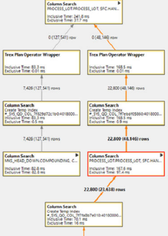
The plan with a shorter execution time (fast case) is shown below:
86 P U B L I C
SAP HANA Performance Guide for Developers
SQL Query Performance
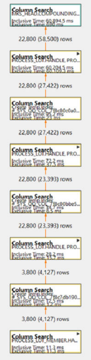
The plan with a longer execution time (slow case) is shown below:
SAP HANA Performance Guide for Developers
SQL Query Performance
P U B L I C 87
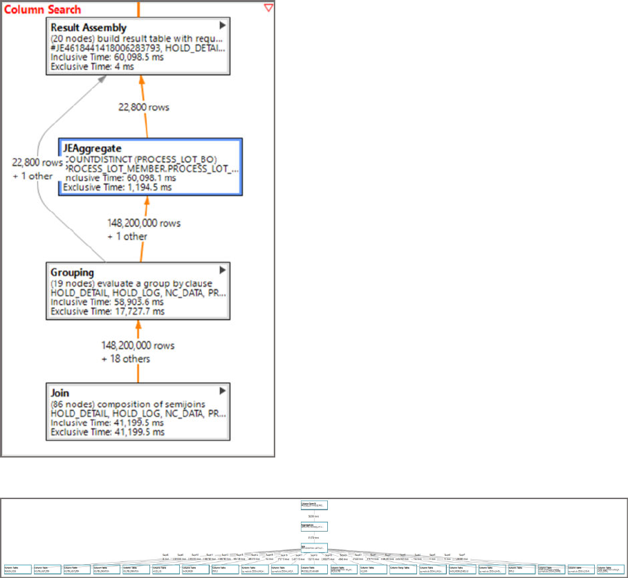
First you need to try to nd a hot spot, which is the point with the longest exclusive execution time. In the slow
case, 60.1 seconds out of 60.9 seconds are required for the second last column search. To see this more
clearly, you can expand the column search by using the downward arrow in the top right corner.
In the expanded version of the heaviest column search (slow case), you can see that there is a join that takes 41
seconds and produces 148 million rows, which are then aggregated for another 17 seconds:
The logical plan of this join shows that 14 dierent tables are joined at once:
The two plans show that although the data size is small before and after the column search, there is a huge
intermediate result inside the column search between the aggregation and the join. You can only see this by
expanding the thread. The heavy complex join is the root cause of the large amount of intermediate data and
the performance degradation. The same joins and aggregations exist in the fast case too, but they are dierent.
In the very rst gure above, the red box is the equivalent part of the joins and aggregations in the fast case.
To compare the two more easily, you might want to simplify the structure of the statement and create diagrams
of the join conditions and the numbers of resulting rows, as shown below. The big boxes contain the join
operators with their join conditions, including the join type and the coordinates of the relation and column. The
numbers between the boxes are the estimated sizes of the intermediate result.
88
P U B L I C
SAP HANA Performance Guide for Developers
SQL Query Performance
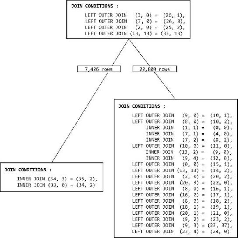
A simplied diagram of the joins in the fast case is shown below:
SAP HANA Performance Guide for Developers
SQL Query Performance
P U B L I C 89
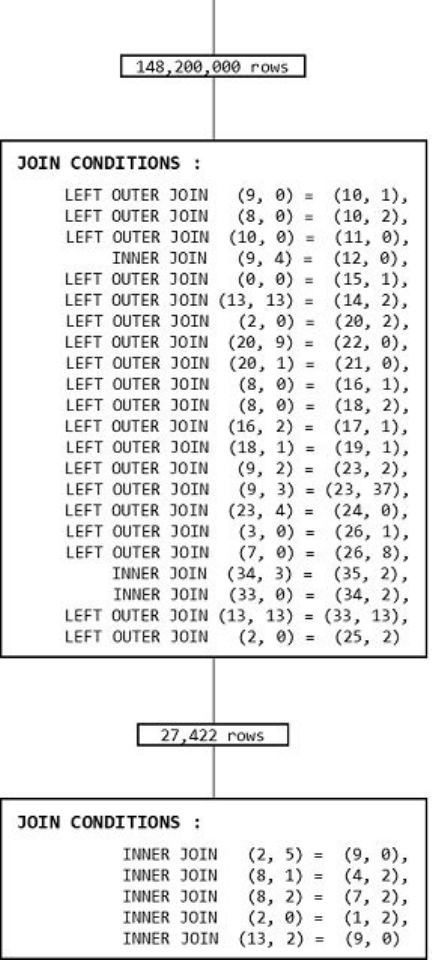
A simplied diagram of the joins in the slow case is shown below:
By comparing the two diagrams, you can easily see that the two inner joins of (34, 3)=(35,2) and (33,0)=(34,2)
are done separately in the fast case whereas they are absorbed into the later column search in the slow case.
Since these two joins were already done beforehand in the fast case, the next column search does not have to
hold so much data and has a reduced number of joins (4) and therefore reduced complexity. To ensure that the
statement always uses the fast plan and does not to fall back to the slow plan, you should force it to not push
down the joins because otherwise the joins will be absorbed into the huge column search whenever possible. To
do this, enumeration rules could help.
The performance uctuation, which is the main issue in this scenario, is caused by the uctuating data. The
SQL optimizer is sensitive to the size of the data. Therefore, varying data sizes can diminish the level of
consistency in execution performance. Such issues arise particularly when the data size oscillates around
90
P U B L I C
SAP HANA Performance Guide for Developers
SQL Query Performance

several internal thresholds that the optimizer uses. One way to make the performance consistent is to apply a
hint that can ensure that the fast plan is chosen.
5.4.1.3 Execution Engines
There are three very similar SQL statements that use the same view as their source. Although they are very
similar, their levels of performance are very dierent.
For example, Query1 takes around 30 times longer than Query2 although the only dierence between them is
their aggregated columns. Also, Query2 is 15 times faster than Query3 even though the former is an
aggregation of the latter. The logic behind these statements needs to be analyzed.
Statements
-- Query1: 6 seconds
-- executed in CALC engine
SELECT DISTINCT COUNT(CASE_KEY)
FROM "SCHEMA"."CALCULATION_VIEW"
WHERE "ID" = '002';
-- Query2: 236 ms
-- executed in OLAP engine
SELECT DISTINCT COUNT(ID)
FROM "SCHEMA"."CALCULATION_VIEW"
WHERE "ID" = '002';
-- Query3: 3 seconds
-- executed in JOIN engine
SELECT ID
FROM "SCHEMA"."CALCULATION_VIEW"
WHERE "ID" = '002';
Analysis
The most obvious dierence seen in Query3 is that it does not have any aggregation or group by operations. If a
query string does not have any aggregations, the OLAP engine will not be responsible for any part of the
execution because it is designed to operate only when there is an aggregation. (The presence of one or more
aggregations, however, does not guarantee that the OLAP engine will be used.) Externally, Query2 seems more
complex than Query3 because it has an additional operation, which is an aggregation. Internally, however, it is
highly likely that the OLAP engine would take care of the operation of Query2. Since the OLAP engine can
demonstrate a very high level of performance particularly when a query contains aggregations with no complex
expressions or functions, Query2 took 0.2 seconds while Query3 took 3 seconds.
SAP HANA Performance Guide for Developers
SQL Query Performance
P U B L I C 91
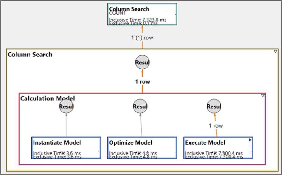
The visualized plan of Query1 is shown below:
92 P U B L I C
SAP HANA Performance Guide for Developers
SQL Query Performance
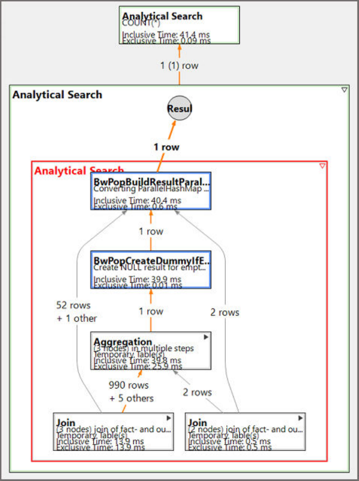
The visualized plan of Query2 is shown below:
SAP HANA Performance Guide for Developers
SQL Query Performance
P U B L I C 93
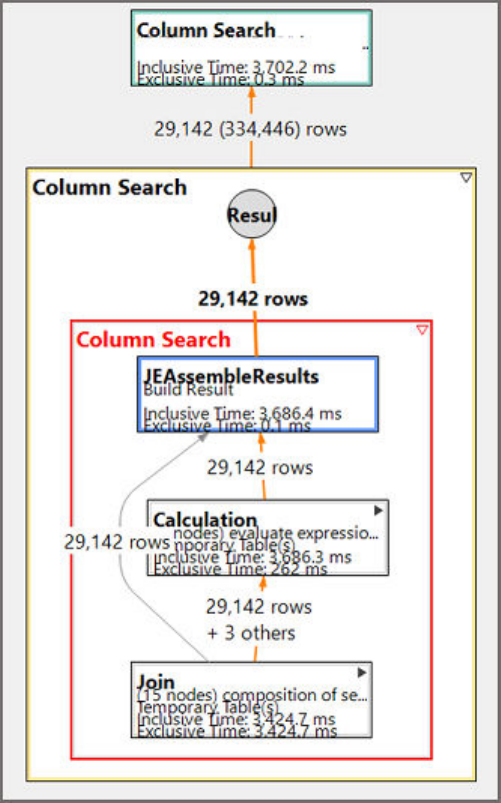
The visualized plan of Query3 is shown below:
Another analysis involves a comparison between Query1 and Query2. The only dierence between them is the
aggregated column. As mentioned above, the presence of an aggregation in the query string does not
necessarily mean that the OLAP engine will be responsible for executing the query. There can be situations
where OLAP execution is blocked due to a limitation such as too little data in the data source. Another reason
why the OLAP engine might not be used could be that the plan was not unfolded in the case of a calculation
view. As explained in previous sections, calculation views are unfolded by default except in certain cases when
there are unfolding blockers or missing features. If unfolding is blocked, the whole optimization task of the SQL
optimizer is handed over to the calculation engine. The calculation engine then executes the operation instead
of the OLAP engine. That is exactly what happened in the case of Query1. Due to calculation view unfolding
blockers, the view was not unfolded, which meant that it could not be processed by the OLAP engine. As a
result, it had to be processed by the calculation engine.
The analysis of the dierent levels of performance of the three queries has shown that their behavior and
performance can be very dierent to what you might expect when the queries are simply viewed from the
outside. Also, it is not a simple rule but a set of complex calculations that determine which engine takes on
which operations, so it is not always predictable which engine will be used for a certain task. More importantly,
one execution engine is not better than another in every situation. Dierent engines exist for dierent
94
P U B L I C
SAP HANA Performance Guide for Developers
SQL Query Performance

purposes. There is therefore no need to question the validity or capacity of the execution engine selected to
execute the generated plan.
5.4.2 Performance Fluctuation of an SDA Query with UNION
ALL
The performance of an identical statement ranges from 0.5 seconds to 90 seconds. The system is a scale-out
system with more than 10 nodes with a remote data source connected through Smart Data Access (SDA).
The query statement is a SELECT statement on a calculation view which consumes SDA virtual tables with
UNION ALL, INNER JOIN, and AGGREGATION operations on those sources. Depending on how much data is
contained in the table and which variants are used for the query, the query transmitted to the remote source
changes. This change has a signicant impact on the overall performance. The best option needs to be found
to minimize the performance uctuation and ensure that the query is always fast.
Statements
SELECT query on the main node
SELECT
sum("COLUMN_1") AS "COLUMN_1 ",
sum("COLUMN_2") AS "COLUMN_2",
sum("COLUMN_3") AS "COLUMN_3",
sum("COLUMN_4") AS "COLUMN_4",
sum("COLUMN_5") AS "COLUMN_5",
sum("COLUMN_6") AS "COLUMN_6",
sum("COLUMN_7") AS "COLUMN_7",
sum("COLUMN_8") AS "COLUMN_8",
sum("COLUMN_9") AS "COLUMN_9",
sum("COLUMN_10") AS "COLUMN_10",
sum("COLUMN_11") AS "COLUMN_11",
sum("COLUMN_12") AS "COLUMN_12",
sum("COLUMN_13") AS "COLUMN_13",
sum("COLUMN_14") AS "COLUMN_14"
FROM "SCHEMA"."VIEW_ABCD"
('PLACEHOLDER' = ('$$INPUT_PARAM$$', '''ZAAA'''))
where "SALESORG" = '1000' and "CALDAY" between '20190101' and '20191231';
The query created and transmitted to the remote source through SDA
SELECT
SUM("VIEW_ABCD"."COLUMN_1"),
SUM("VIEW_ABCD"."COLUMN_2"),
SUM("VIEW_ABCD"."COLUMN_3"),
SUM("VIEW_ABCD"."COLUMN_4"),
SUM("VIEW_ABCD"."COLUMN_5"),
SUM("VIEW_ABCD"."COLUMN_6"),
SUM("VIEW_ABCD"."COLUMN_7"),
SUM("VIEW_ABCD"."COLUMN_8"),
SUM("VIEW_ABCD"."COLUMN_9"),
SUM("VIEW_ABCD"."COLUMN_10"),
SUM("VIEW_ABCD"."COLUMN_11"),
SUM("VIEW_ABCD"."COLUMN_12"),
SUM("VIEW_ABCD"."COLUMN_13"),
SAP HANA Performance Guide for Developers
SQL Query Performance
P U B L I C 95
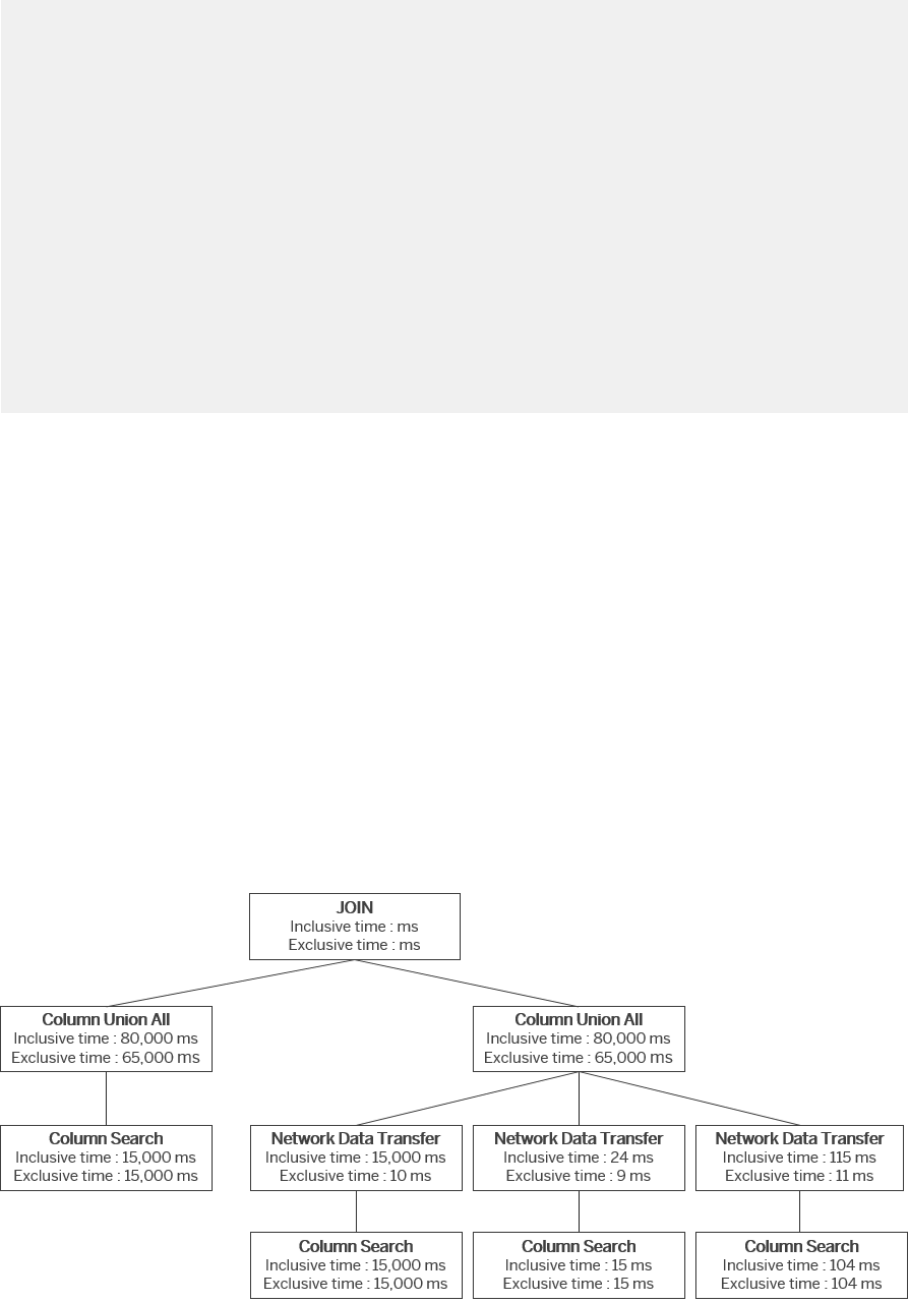
SUM("VIEW_ABCD"."COLUMN_14")
FROM (SELECT
"COLUMN_1",
"COLUMN_2",
"COLUMN_3",
"COLUMN_4",
"COLUMN_5",
"COLUMN_6",
"COLUMN_7",
"COLUMN_8",
"COLUMN_9",
"COLUMN_10",
"COLUMN_11",
"COLUMN_12",
"COLUMN_13",
"COLUMN_14
FROM "_SYS_BIC"."Model.Package/VIEW_ABCD"
( PLACEHOLDER."$$INPUT_PARAM$$" => '''ZAAA''' ) ) "VIEW_ABCD"
WHERE "VIEW_ABCD"."SALESORG" = '1000'
AND "VIEW_ABCD"."CALDAY" >= '20190101'
AND "VIEW_ABCD"."CALDAY" <= '20191231';
Related Information
Initial Analysis [page 96]
Apply the Hint NO_CS_UNION_ALL [page 98]
Reinvestigate the Visualized Plan from an Overall Perspective [page 99]
Case-Study Conclusions [page 103]
5.4.2.1 Initial Analysis
You can use the Plan Visualizer to compare the plan that runs in a short time (good plan) with the plan with a
longer execution time (bad plan).
The visualized plan of the bad plan is shown below:
96
P U B L I C
SAP HANA Performance Guide for Developers
SQL Query Performance
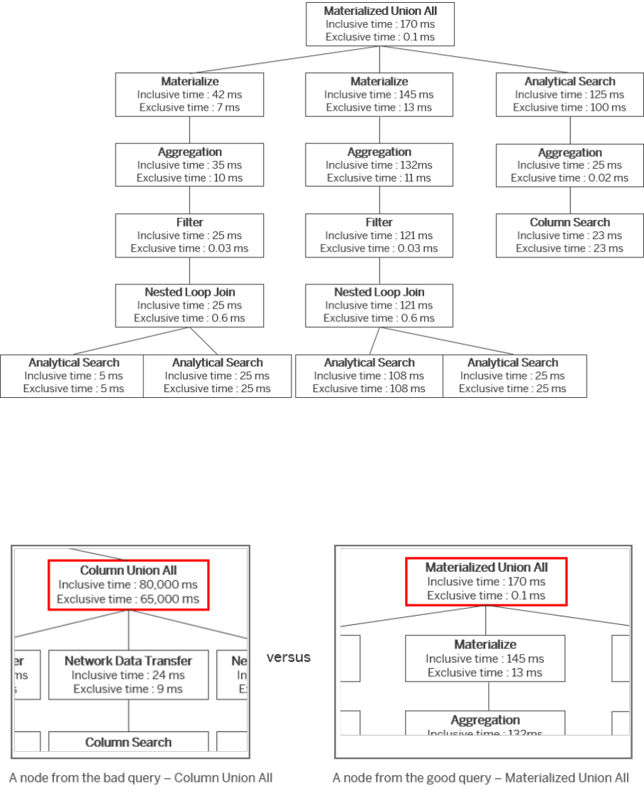
The visualized plan of the good plan is shown below:
The plans are obviously dierent, but they do not help you to pinpoint the operations which were changed into
other operations. Since the problem is a long execution time, you should start by nding the spot in the
execution plan that caused the long execution time. In the bad plan, it is Column Union All, which required 65
seconds out of the 80 seconds of inclusive time.
You can see that dierent algorithms are used in the UNION operation. The bad plan uses Column Union All
whereas the good plan uses Materialized Union All:
You should not conclude that Materialized Union All is a faster operator than Column Union All. In many cases,
particularly when complex business data is stored in column store tables as numbers, column operators run
better than row operators. This can be conrmed in the next step, where you apply the hint
NO_CS_UNION_ALL.
SAP HANA Performance Guide for Developers
SQL Query Performance
P U B L I C 97
5.4.2.2 Apply the Hint NO_CS_UNION_ALL
Because you can see that the dierent physical Union All operators result in dierent performance, you can try
applying the hint NO_CS_UNION_ALL, which adds more weight to the row operator when the SQL optimizer
processes the physical enumeration step of Union All.
Unless the estimated benet of the column operator outweighs the additional weight given to the row operator,
the hint will force the Materialized Union All operator to be chosen. The real-case scenario beneted from the
application of this hint and saw a considerable improvement in the execution performance.
Note that this solution was particular to that scenario. Simply changing the physical operator from column to
row is often not very helpful. This is mainly because one of the SQL optimizer's features is to prefer column
operators by default so as to benet from a fully columnar plan. By making the plan into one single column
search, no materialization is involved, and performance is expected to improve. Therefore, the optimizer
prefers to use columnar operators and push them into column searches whenever it can.
With respect to the optimizer’s preference for column operators, further analysis should be done to identify the
fundamental scope and root cause.
98
P U B L I C
SAP HANA Performance Guide for Developers
SQL Query Performance
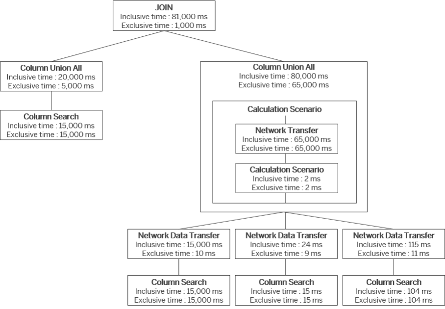
5.4.2.3 Reinvestigate the Visualized Plan from an Overall
Perspective
Instead of viewing the Plan Visualizer in the way it is initially presented, you can drill down the column search
operators by clicking the downward arrows. This gives you much more information not only about the
execution engines but also about the operations that are hidden at rst glance.
The visualized plan of the bad plan with Column Union All unfolded is shown below:
SAP HANA Performance Guide for Developers
SQL Query Performance
P U B L I C 99
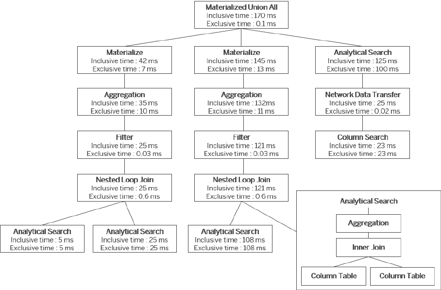
The visualized plan of the good plan with one of the Analytical Searches unfolded is shown below:
By expanding the column searches, you can see the overall structure of the plan.
The visualized plan of the bad plan with estimated data sizes is shown below:
100
P U B L I C
SAP HANA Performance Guide for Developers
SQL Query Performance
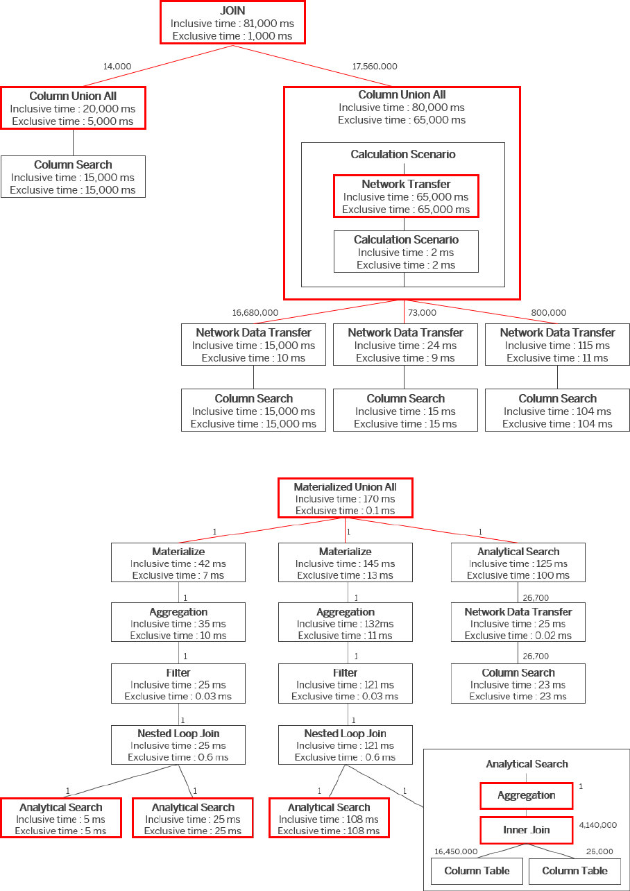
The visualized plan of the good plan with estimated data sizes is shown below:
SAP HANA Performance Guide for Developers
SQL Query Performance
P U B L I C 101
In the bad plan, Column Union All took 65 seconds out of the total execution time of 80 seconds, and most of
the 65 seconds were consumed by the operation called Network Data Transfer. Network Data Transfer occurs
when the data is in another node of the system and needs to be transferred through the network to another
node for further processing. Considering that the same Network Data Transfers already happened at the
beginning to fetch the data from the base tables, this plan involves a heavy network load compared to that seen
in the faster plan. The location of the operation is determined internally in the SQL optimizer, using multiple
values as its variables. It is therefore very dicult to relocate just this one operation to another location without
aecting other operations. Therefore, you need to nd a more fundamental reason as to why these operations
had to be transferred and why they caused such a signicant performance degradation.
The big dierence between the two plans is that the good plan has the Union operation after the joins, whereas
the bad plan has the Union operations before the join. In the good plan, the INNER JOINs are under the
Analytical Search (column search of the OLAP engine), which is hidden when it is collapsed. Moreover, the good
plan is even faster due to the AGGREGATIONs that are located right after the table scans. In the Analytical
Search at the bottom, the data is already aggregated with a single record as the intermediate result, which is
extremely helpful for reducing the execution time. The other Analytical Searches share the same structure,
which means there are already four AGGREGATIONs and four INNER JOINs before the Materialized Union All
operation is reached.
On the other hand, there is nothing signicant inside the base Column Searches of the bad plan, but there is a
calculation scenario inside Column Union All. Apart from the fact that this means that this part of the plan
could not be unfolded and had to be handled by the calculation engine, a calculation scenario can involve a
large complex model which generally has many aggregations, joins, and expressions. Therefore, it is highly
probable that the bad plan's counterparts of AGGREGATIONs and INNER JOINs are inside the calculation
scenario. In the real case scenario, there were multiple aggregations in the calculation model. The location of
these aggregations and joins matters because intermediate data sizes cannot be reduced if those operations
are not done at the beginning of the execution. When the heavy operations are performed later, the size of the
intermediate results is larger, which results in a slower performance.
Overall, therefore, the dierence in the logical structure is a potential cause of the performance degradation.
Consequently, you could decide to apply hints that would push down the joins through the Union All operation
and even the aggregations as well.
Apply Hint PREAGGR_BEFORE_UNION
There are many hints that you could try applying. They include PREAGGR_BEFORE_JOIN, AGGR_THRU_JOIN,
PREAGGR_BEFORE_UNION, and JOIN_THRU_UNION. You could select a single hint or combine hints from this
list and then test the resulting performance.
In the real-case scenario, PREAGGR_BEFORE_UNION was suciently eective on its own because the
aggregations produced just one record, which is a cardinality that can improve the entire query performance.
When data is aggregated at an earlier stage, a greater performance gain is expected, which was conrmed by
the considerable performance improvement seen when the aggregations were positioned before the joins.
102
P U B L I C
SAP HANA Performance Guide for Developers
SQL Query Performance

5.4.2.4 Case-Study Conclusions
These were the key takeaways from this case study.
● The Plan Visualizer is the starting point in most cases.
Although the Plan Visualizer is not a perfect tool and it does not contain all the information that you might
need, it is the best tool for getting an analysis started on the right track. Since it uses a visualized format, it
is much easier to understand compared to other traces and it allows you to get a better overview of the
entire process. You can drag the plan to see its overall shape. The node colors help you to more precisely
compare plans when you have multiple plans. Even if you know that the Plan Visualizer will not help you to
nd the actual solution, you should still start o with the Plan Visualizer to ensure your eorts are focused
in the right direction.
● There is no single answer for solving these problems.
Even though you have potential workarounds that seem to work on a specic scenario, you can never know
which one or which combination will work before you test them on the query. The plans are complicated,
and in most cases you will not be able to correctly predict how the hints will work. SQL optimization is not
simple math and it takes numerous comparisons, calculations, and evaluations to reach the nal decision.
You should never rely on suggested workarounds until they are proven to work in the production system.
5.4.3 Composite OOM due to Memory Consumed over 40
Gigabytes by a Single Query
A single query runs forever and does not return any results. With the statement memory limit set to 40
gigabytes, the query execution ends up with a composite out-of-memory error. Such behavior was rst seen a
few days ago and since then it happens every time the query runs.
You need to nd the root cause and a solution.
Statement
SELECT
/* FDA READ */ /* CDS access control applied */ "COMPANYCODE" ,
"ACCOUNTINGDOCUMENT" ,
"FISCALYEAR" ,
"ACCOUNTINGDOCUMENTITEM" ,
"TAXCODE" ,
"TRANSACTIONTYPEDETERMINATION" ,
"STATRYRPTGENTITY" ,
"STATRYRPTCATEGORY" ,
"STATRYRPTRUNID" ,
"TAXNUMBER1" ,
"COUNTRY" ,
"DEBITCREDITCODE" ,
"TAXCALCULATIONPROCEDURE" ,
"TAXRATE" ,
"IPITAXRATE" ,
"ADDITIONALTAX1RATE" ,
"CONDITIONAMOUNT" ,
"CUSTOMER" ,
"GLACCOUNT" ,
SAP HANA Performance Guide for Developers
SQL Query Performance
P U B L I C 103

"TAXITEMGROUP" ,
"BUSINESSPLACE" ,
"TAXJURISDICTION" ,
"LOWESTLEVELTAXJURISDICTION" ,
"ACCOUNTINGDOCUMENTTYPE" ,
"REFERENCEDOCUMENTTYPE" ,
"REVERSEDOCUMENT" ,
"REVERSEDOCUMENTFISCALYEAR" ,
"CONDITIONRECORD" ,
"ROUNDINGDECIMALPLACES" ,
"DOCUMENTREFERENCEID" ,
"LEDGER" ,
"LEDGERGROUP" ,
"POSTINGDATE" ,
"DOCUMENTDATE" ,
"TAXREPORTINGDATE" ,
"REPORTINGDATE" ,
"FISCALPERIOD" ,
"EXCHANGERATE" ,
"ISREVERSAL" ,
"ACCOUNTINGDOCUMENTHEADERTEXT" ,
"COMPANYCODECOUNTRY" ,
"REPORTINGCOUNTRY" ,
"DIFFERENCETAXAMTINCOCODECRCY" ,
"DIFFTAXBASEAMOUNTINCOCODECRCY" ,
"TAXTYPE" ,
"TARGETTAXCODE" ,
"TAXNUMBER2" ,
"ACTIVETAXTYPE" ,
"TAXNUMBER3" ,
"CALCULATEDTXAMTINCOCODECRCY" ,
"CALCULATEDTAXAMOUNTINTRANSCRCY" ,
"BUSINESSPARTNER" ,
"CALCDTXBASEAMTINCOCODECRCY" ,
"CALCULATEDTXBASEAMTINTRANSCRCY" ,
"TOTALGROSSAMOUNTINCOCODECRCY" ,
"TOTALGROSSAMOUNTINTRANSCRCY" ,
"NONDEDUCTIBLEINPUTTAXAMOUNT" ,
"CONFIGURATIONISACTIVE" ,
"TRIGGERISACTIVE" ,
"DCBLVATINCRDCOSTINRPTGCRCY" ,
"BUSINESSPARTNERNAME" ,
"TAXTYPENAME" ,
"CUSTOMERSUPPLIERADDRESS" ,
"TAXISNOTDEDUCTIBLE" ,
"BALANCEAMOUNTINTRANSACCURRENCY" ,
"CONDITIONTYPE"
FROM /* Entity name: I_STRPTAXRETURNCUBE CDS access controlled */
"ISRTAXRETURNC" ( "P_ISPARAMETER" => 'N' , "P_CONDITIONISMANDATORY" => 'N' )
"I_STRPTAXRETURNCUBE"
WHERE "MANDT" = '100';
Related Information
Plan Visualizer Overview [page 105]
Filter Pushdown to Other Join Candidates [page 105]
Columnize the Filter [page 106]
Push Down the Aggregation Through the Joins [page 107]
Case-Study Conclusions [page 108]
104
P U B L I C
SAP HANA Performance Guide for Developers
SQL Query Performance
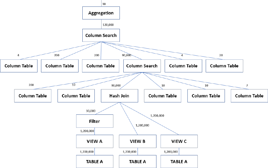
5.4.3.1 Plan Visualizer Overview
Use the Plan Visualizer to start o your analysis.
The Plan Visualizer overview of the badly performing query is shown below:
You can see that the views VIEW A, VIEW B and VIEW C share the same base table (TABLE A) as their data
source. The join between the three views is followed by another join with ve other tables, and then yet another
join, which is followed by an aggregation. These joins involve multiple tables, but the data size of each table is
not that big. It therefore seems strange that this query should have a memory problem.
5.4.3.2 Filter Pushdown to Other Join Candidates
The lter applied to VIEW A is pushed down from one of the parent nodes. For example, you position this lter
after the join between VIEW A, VIEW B, and VIEW C, and then this lter can be pushed down to the join
candidates depending on their join conditions.
In this case, only VIEW A inherited the lter, even though the three views have the same base table as the data
source. If you could therefore push down the same lter to the other two views as well, the join size could be
reduced dramatically. In the current situation, the maximum joined data size is 43.2 quadrillion (30,000 *
1,200,000 * 1,200,000 = 43,200,000,000,000,000). If you could reduce the data from the other two views, it
could be lowered to 27 trillion (30,000 * 30,000 * 30,000 = 27,000,000,000,000). This is a huge improvement
with the data size reduced by more than a factor of a thousand.
SAP HANA Performance Guide for Developers
SQL Query Performance
P U B L I C 105
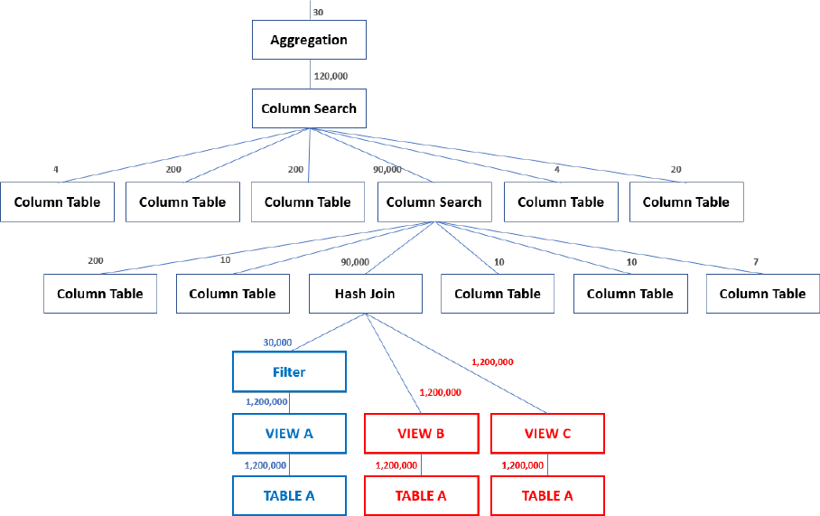
Consider lter pushdown to TABLE A, which is used repeatedly by dierent views:
You could consider altering some of the join conditions to force the lter to be pushed down to the other two
views. In the real case scenario, this was solved by adding one join condition for each relation (VIEW A to VIEW
B, and VIEW A to VIEW C). The column used in this join condition was the ltered column in VIEW A. In this way,
the lter could be pushed down from the parent node and even from one join candidate to another.
5.4.3.3 Columnize the Filter
Another aspect to think about is changing the physical operators. Although all the source tables used in this
query are column-store tables, several row operators are used.
This is not "wrong" because if there is a column-search blocker, such as in VIEW A in this scenario, the logical
decision would be to execute the subsequent operations in row engines. However, if these operators were
executed in column engines and potentially even absorbed into existing column searches, this would make the
structure completely dierent. If the lter in the diagram below were changed into a column operator, it is
highly likely that it would be absorbed into the column search, and the existing column searches merged into
one or two.
106
P U B L I C
SAP HANA Performance Guide for Developers
SQL Query Performance
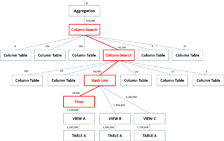
Consider columnizing the lter:
In the real case scenario, the row lter was turned into a columnar one by applying the hint CS_FILTER, which
actually reduced the memory usage of the query. The query required 2 minutes, which was still not entirely
satisfactory, but the main goal of avoiding composite memory was achieved.
5.4.3.4 Push Down the Aggregation Through the Joins
The aggregation at the end of the plan is very eective because it reduces 120,000 rows to 30 rows. However,
there is no reason why an eective data reducer needs to be positioned at the end of the plan, where the data
reduction might no longer be very signicant.
It might be better to push down the aggregation below the joins to minimize the intermediate result as much as
possible. The intermediate result size is a critical factor when it comes to huge memory usage problems.
In the real case scenario, the hint NO_JOIN_THRU_AGGR was used together with the hint CS_FILTER. This
combination reduced the execution time to 29.6 seconds.
SAP HANA Performance Guide for Developers
SQL Query Performance
P U B L I C 107
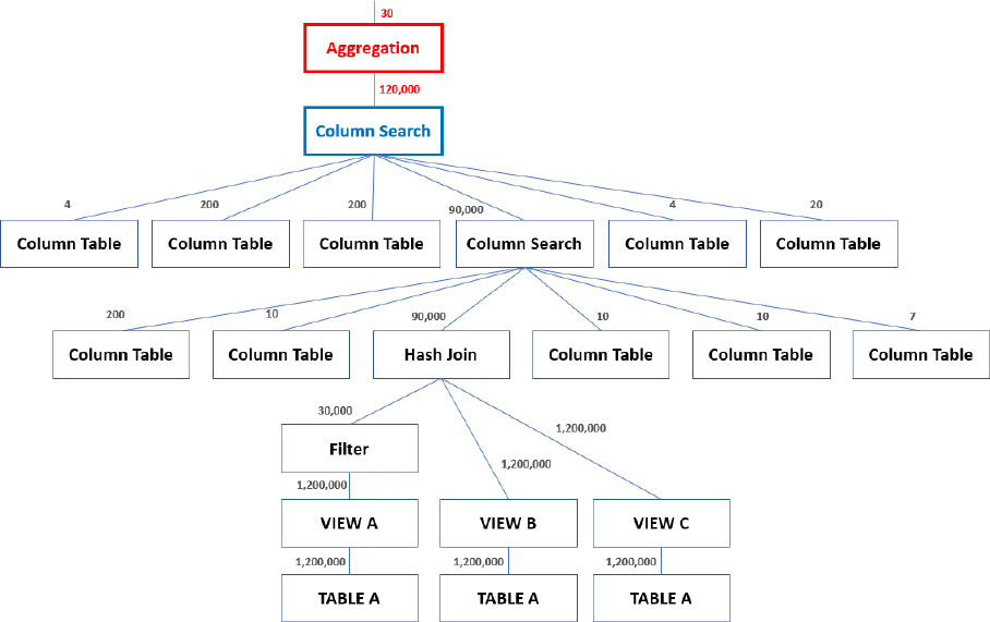
Consider pushing down the aggregation through the joins:
5.4.3.5 Case-Study Conclusions
These were the key takeaways from this case study.
● For memory problems, the key is to reduce the intermediate result.
Even when the datasets of join candidates are small, the result can be huge when they are multiplied. This
is a problem particularly when the join is an inner join, because inner joins do not guarantee data reduction
after the join. In the worst case, the intermediate result is the cross product between the candidates.
The rst step to minimize the intermediate results is to try adding more lters. It is best to change the
statement or use ALTER commands to modify the denition of the views. However, there are cases where
you cannot modify the denitions because some of the objects are standard objects which cannot be
changed. Nevertheless, you still can modify the plan by changing the factors around those standard
objects. A good example is to add join conditions for lter pushdown as shown above.
● It is worth thinking about the physical operators that are used.
In general, one operator is not better than another, so it might be helpful to consider which physical
operator is more ecient for a given situation. For example, the tables used are mostly column-store
tables. If there is no clear evidence why the row operators are needed in the plan, it is worth putting more
weight on column engines, because that would allow the benets of absorption to be utilized.
108
P U B L I C
SAP HANA Performance Guide for Developers
SQL Query Performance

5.4.4 Performance Degradation of a View after an Upgrade
Caused by Calculation View Unfolding
After an upgrade, one of the calculation views is slower than before the upgrade, while other views have an
overall performance gain. The problematic view is a standard SAP HANA model, so changes to this model are
not allowed.
The main dierence which can be easily seen is that plan is unfolded in the upgraded system whereas it was
not unfolded in the previous revision. This is because calculation views are unfolded by default unless they are
congured otherwise or they cannot be unfolded. Generally, calculation view unfolding allows a better
optimization to be achieved, but it does not seem to be the case in this scenario. You want to restore the
previous level of performance or at least mitigate the performance degradation in the current version.
Statement
select * from "_SYS_BIC"."sap.is.ddf.dc/DistributionCurveQuery"(
PLACEHOLDER."$$P_SAPClient$$" => '100',
PLACEHOLDER."$$P_TaskId$$" => '01',
PLACEHOLDER."$$P_PlanningDate$$" => '20190101');
Related Information
Overview of a Complex Execution Model [page 109]
Hot Spot Analysis [page 111]
Operation Detail Analysis [page 112]
Plan Analysis [page 113]
Case-Study Conclusions [page 115]
5.4.4.1 Overview of a Complex Execution Model
The execution plan at issue is extremely complex when displayed in the Plan Visualizer trace. However, it worth
remembering that the Plan Visualizer is a good starting point because it is one of the least complex traces.
To get started, it is most important to nd the hot spot. The hot spot is the operation with the longest execution
time. In the real case scenario, there were two main points that required most of the execution time. You should
therefore start o by focusing on these two points, enlarging the area around them, and simplifying the
components to see what is happening.
SAP HANA Performance Guide for Developers
SQL Query Performance
P U B L I C 109
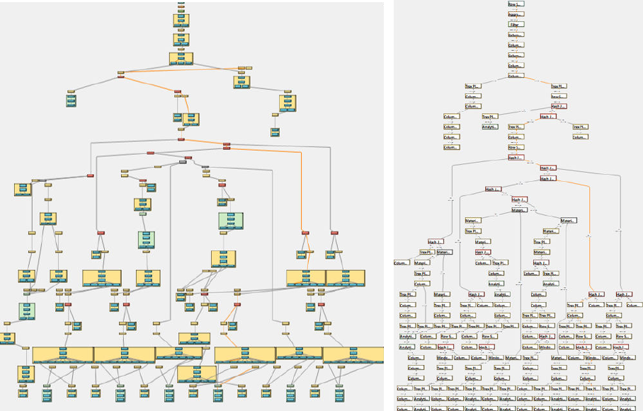
The whole visualized plan for this case, expanded (left) and collapsed (right), is shown below:
110 P U B L I C
SAP HANA Performance Guide for Developers
SQL Query Performance
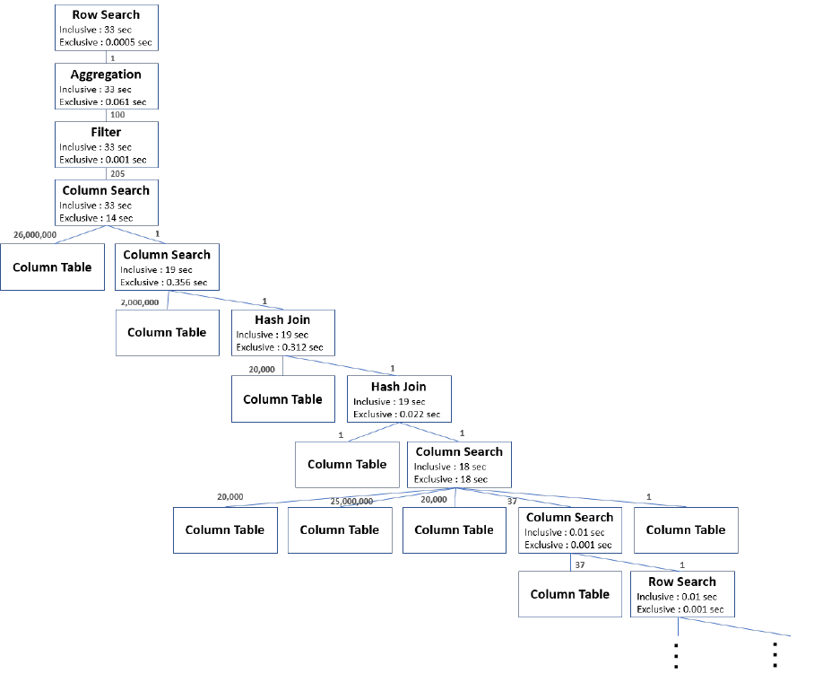
5.4.4.2 Hot Spot Analysis
While the entire plan takes 33 seconds to execute, most of this execution time involves the later part of the
execution, which is shown by the operators at the top of the visualized plan.
This upper part of the graph is magnied as shown below:
If you look more closely at this part, you can see that there are two column searches that consumed most of
the time, 14 seconds and 18 seconds, respectively. Considering that the total execution time was 33 seconds,
the query would gain hugely in performance if these two knots were removed.
The logical structure shows that both column searches at issue are joins. As in the previous case study, you
should try to work out what happened by looking at the join candidates' data sizes. However, in this case the
join candidates are not heavy. One of the join candidates of the 14-second column search only has a single
record. The join of the 18-second column search involves ve dierent tables as join candidates, but they are
not very big. Also, the output of this join is just one record, which implies that the cardinality of this join must
have been very small.
It is therefore strange that these two joins took so long to be completed. To investigate further, you need to look
at the details of the join operations.
SAP HANA Performance Guide for Developers
SQL Query Performance
P U B L I C 111
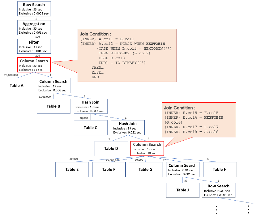
5.4.4.3 Operation Detail Analysis
The operation details normally include the operator name, its internal ID, schema, exclusive and inclusive
execution times, execution start and end times, and other detailed information depending on the type of
operation. For joins, it shows the join type, conditions, and cardinality.
To see the operation details, you just need to hover over the operator.
The upper part of the visualized plan under investigation is shown again with the operation details added on the
side:
The rst join from the top of the two previously mentioned joins has two inner join conditions, "A.col1 = B.col1"
and "A.col2 = NCASE WHEN HEXTOBIN (CASE WHEN…". While the rst condition is quite simple, the second
condition contains multiple layers of evaluation. These evaluations also contain expressions like HEXTOBIN(),
BINTOHEX(), and TO_BINARY().
Normally, multiple layers of CASE do not cause any problems. Depending on the situation, however, the CASE
predicate can play a role as a pushdown blocker, but just because there are many CASEs, this does not
necessarily mean that they should be rewritten or xed. The expressions that are used to alter the values into
dierent text types are more worthy of attention. Turning hexadecimal codes into binaries and vice versa
requires the actual value of each row in the column to be expressed in the target type. This is a row-wise
112
P U B L I C
SAP HANA Performance Guide for Developers
SQL Query Performance
process that needs to be done by reading the value of each individual row. In this context, it does not seem
appropriate that these expressions are processed in the column engines, as seen in the case scenario. It is not
clear what the benet would be of a columnar operation in this situation.
The reason behind this is that row-wise expressions have, over time, acquired columnar counterparts. At rst,
these expressions probably only existed as row engine operators and therefore probably served as pushdown
blockers and undermined the chance of building columnar plans. To tackle those situations, equivalent
expressions were built on the column engine side, too. In this particular case, it is likely that column
expressions are chosen and pushed down because the SQL optimizer prefers column operations to row
operations.
It is worth trying the hint NO_CS_EXPR_JOIN because this will remove the weight on the column engine when
the physical operators are determined for the expression joins. The NO_CS_EXPR_JOIN hint could also have a
positive eect on the other heavy join, which also has a row-wise expression (HEXTOBIN).
In the real case scenario, NO_CS_EXPR_JOIN cut the execution time down to a quarter of its previous length,
that it, to around 9 seconds. With the hint applied, the upper join that originally took 14 seconds was reduced to
less than one second, and the other join requiring 18 seconds was reduced to 5 seconds.
5.4.4.4 Plan Analysis
An additional improvement point was found by looking at the plan from some distance. The plan is very big and
complex, with heavily repeated joins and aggregations. The joins and aggregations in this plan were mostly
executed by the join engine (column search) and row engine (hash join).
In SAP HANA, repeated joins with aggregations are often assigned to the OLAP engine because it is good at
bringing together large datasets particularly when they are in a fact-and-dimension relationship. However, in
this scenario, OLAP operations (analytical search) were rare.
The lower part of the visualized plan is shown below:
SAP HANA Performance Guide for Developers
SQL Query Performance
P U B L I C 113
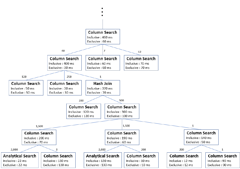
Although the beginning of the plan does not require much time, there is still room for improvement, which is
evident when you capture the pattern in the logical structure. The estimated sizes of the output after each
operation are all less than 5,000. By default, OLAP engines can process aggregations when the input data has
over 5,000 rows. In other words, when aggregations have an input data size that is smaller than 5,000, the SQL
optimizer does not even consider using the OLAP engine to execute them. This means that the plans with small
datasets cannot utilize the benets of the OLAP engine even when it would be benecial. The decision rule for
deciding between the OLAP engine or the join engine is designed to make the compilation process more
eective and allows the SQL optimizer to avoid redundancy. From time to time, you might need to intervene,
depending on the situation.
To make the SQL optimizer consider the OLAP engine for join and aggregation executions even with small
datasets, you can try using the hint USE_OLAP_PLAN. In the real case scenario, the hint USE_OLAP_PLAN
together with the hint NO_CS_EXPR_JOIN reduced the total execution time to 7 seconds.
114
P U B L I C
SAP HANA Performance Guide for Developers
SQL Query Performance
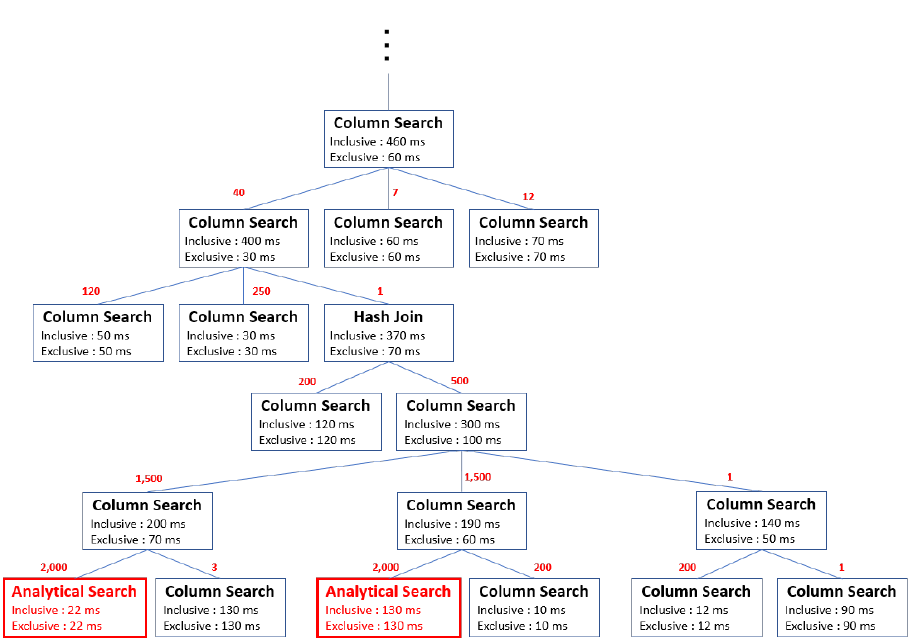
The lower part of the visualized plan with the estimated sizes highlighted is shown below:
5.4.4.5 Case-Study Conclusions
These were the key takeaways from this case study.
● It is worth trying dierent column engines.
There are various rules that help the SQL optimizer decide which engine to use. Some rules are relative
whereas others are absolute. When rules are absolute, they don’t apply under specic conditions or they
are completely blocked. One example, as seen above, is the estimated size of the aggregation input, which
cannot be processed by the OLAP engine when it is under 5,000. In such cases, there are no alternatives to
be compared. Therefore, you need to let the SQL optimizer know that there is an alternative, for example,
that the OLAP engine is an alternative to the join engine. If the SQL optimizer does not respond, this means
that SQL optimizer still thinks the previous alternative is best, even after considering the alternatives you
have just enabled. However, if the SQL optimizer changes its behavior and chooses the alternative, there is
a chance that your workaround could solve the problem. Although there is a risk of performance
degradation after the workaround, it is still worth trying a dierent engine.
● There is no magic word in performance tuning.
Finding the problematic expressions out of tens of operators in the Plan Visualizer is neither luck nor
intuition. It is time that matters, and the more time you spend analyzing traces, the more information you
will get. There is no magical way to solve a problem, so you should try to read and understand the traces. In
many cases, performance issues can be mitigated by using simple hints.
SAP HANA Performance Guide for Developers
SQL Query Performance
P U B L I C 115

Whenever there is a performance issue to solve, it is important to be patient. The Plan Visualizer should be
your rst step, before you move on to all the other resources that are available, and which will enrich your
analysis. Remember to spend time reading and analyzing the trace before jumping to conclusions. You
should always test your solution before implementing it in the production system.
5.5 SQL Tuning Guidelines
You can signicantly improve the performance of SQL queries by knowing how the SAP HANA database and
SAP HANA engines process queries and by adapting them accordingly.
As a general guideline for improving SQL query performance, we recommend avoiding operations that are not
natively supported by the various SAP HANA engines, since they can signicantly increase the time required to
process the queries.
Please note that the specic recommendations described here may help to improve the performance of SQL
queries involving column tables.
Caution
Throughout this section, adding generated columns is mentioned as a possible workaround for improving
query performance. However, it should be noted that adding generated columns improves query
performance at the expense of increased memory consumption, and increased insertion and update cost.
You should be aware of this trade-o before deciding to add generated columns.
5.5.1 General Guidelines
Some basic best practices can help improve the response times of queries on the SAP HANA database.
Select Only Needed Columns
Selecting all columns of an SAP HANA column table will unnecessarily materialize additional columns and
cause memory and CPU overhead.
Avoid Joining Tables of Dierent Types
Joining row and column tables will lead to a table layout conversion and incur a performance penalty.
Restrict this to small data sets if it cannot be avoided.
116
P U B L I C
SAP HANA Performance Guide for Developers
SQL Query Performance

Avoid CRUD Operations in a Loop
Do not perform single record operations (create, read, update, or delete) in a loop on the application level, but
use set operations instead.
One of the strengths of SQL is its set-oriented syntax, which allows entire sets of data (potentially comprising
many individual records) to be fetched and manipulated in a single statement. In most cases, this is also more
ecient than the alternative approach of processing the individual records in a loop and issuing a database
request for each record. Even if a single statement is fast, it adds up over time with the number of operations.
For example, assume you are processing 100,000 records in a loop and performing a database operation on
each of them. If the database operation has a response time of 0.1 milliseconds, you would have an overall
database processing time of 10 seconds. In comparison, if you were to process all the records within a single
database operation, this might require, for example, just 500 milliseconds. This represents a performance
improvement of a factor of 20.
One reason for this dierence is the incompressible overhead which is associated with the communication
between the application server and the database, and the processing within the database. This occurs 100,000
times in the rst case (100,000 individual statements) and only once in the second case (one statement
processes all records).
The following query lists the statements in the SQL plan cache in decreasing order of execution count and can
help you spot statements which were executed many times. Some of the statements might have been executed
in a loop:
SELECT TOP 100 execution_count AS execcount, * FROM m_sql_plan_cache ORDER BY
execution_count DESC;
Use Parameterized Queries
Use query parameters rather than literal values to avoid compiling similar queries multiple times.
5.5.2 Avoiding Implicit Type Casting in Queries
You can avoid implicit type casting by instead using explicit type casting or by adding generated columns.
The system can generate type castings implicitly even if you did not explicitly write a type-casting operation.
For example, if there is a comparison between a VARCHAR value and a DATE value, the system generates an
implicit type-casting operation that casts the VARCHAR value into a DATE value. Implicit type casting is
performed from the lower precedence type to the higher precedence type. For information about the data type
precedence rules, see the SAP HANA SQL and System Views Reference. If two columns are frequently
compared by queries, it is better to ensure that they both have the same data type from the beginning.
One way to avoid the cost of implicit type casting is by using explicit type casting on an inexpensive part of the
query. For instance, if a VARCHAR column is compared with a DATE value and you know that casting the DATE
value into a VARCHAR value produces what you want, it is recommended to cast the DATE value into a
VARCHAR value. If the VARCHAR column contains only date values in the form of 'YYYYMMDD', it could be
compared with a string generated from a DATE value in the form of 'YYYYMMDD'.
SAP HANA Performance Guide for Developers
SQL Query Performance
P U B L I C 117

In the example below, date_string is a VARCHAR column. Note that the result when strings are compared is
generally dierent from the result when dates are compared, and only in some cases is it identical:
Problematic query
SELECT * FROM T WHERE date_string < CURRENT_DATE;
Workaround
SELECT * FROM T WHERE date_string < TO_VARCHAR(CURRENT_DATE, 'YYYYMMDD');
If there is no way to avoid implicit type casting, one way to avoid the issue entirely is to add generated columns.
In the example below, you can nd '1', '1.0', and '1.00' stored in a VARCHAR column using the revised query,
which avoids implicit type casting:
Problematic query
SELECT * FROM T WHERE varchar_value = 1;
Workaround
ALTER TABLE T ADD (num_value DECIMAL GENERATED ALWAYS AS varchar_value);
SELECT * FROM T WHERE num_value = 1;
5.5.3 Avoiding Inecient Predicates in Joins
This section lists the predicate conditions that are not natively supported by the column engine.
Depending on the condition, intermediate results are materialized and consumed by the row engine or column
engine. It is always good practice to try to avoid intermediate result materialization, since materialization can
be costly if results are large and have a signicant impact on the performance of the query.
5.5.3.1 Non-Equijoin Predicates in Outer Joins
The column engine natively supports an outer join with a join predicate of equality. It does not natively support
an outer join with join predicates other than the equality condition (that is, non-equijoin) and join predicates
connected by OR (even if each predicate is an equality condition).
Also, if equijoin predicates are connected to non-equijoin predicates by AND, they are processed in the same
way as cases with only non-equijoin predicates.
When non-equijoin predicates are used, the row engine executes the join operation using the appropriate join
algorithm (nested loop, range, hashed range) after materializing the intermediate results from both children.
118
P U B L I C
SAP HANA Performance Guide for Developers
SQL Query Performance

An example of how a non-equijoin predicate can be rewritten as an equijoin predicate is shown below. In the
example, M is a table containing the rst and last dates of the months of interest:
Problematic query
SELECT M.year, M.month, SUM(T.ship_amount)
FROM T LEFT OUTER JOIN M ON T.ship_date BETWEEN M.first_date AND M.last_date
GROUP BY M.year, M.month;
Workaround
SELECT M.year, M.month, SUM(T.ship_amount)
FROM T LEFT OUTER JOIN M ON EXTRACT(YEAR FROM T.ship_date) = M.year AND
EXTRACT(MONTH FROM T.ship_date) = M.month
GROUP BY M.year, M.month;
5.5.3.2 Calculated Column Predicates
Intermediate results from calculations that are not natively supported by the column engine are materialized,
but this can be avoided by using generated columns.
Most calculations are natively supported by the column engine. If a calculation is not natively supported by the
column engine, the intermediate results from both children are materialized and consumed by the row engine.
One way to avoid this is to add generated columns.
An example of how calculated join columns can be avoided by using generated columns is shown below. In the
example, M is a table containing the rst and last dates of the months of interest:
Problematic query
SELECT * FROM T JOIN M ON NEXT_DAY(T.ship_date) = M.last_date;
Workaround
ALTER TABLE T ADD (next_day DATE GENERATED ALWAYS AS ADD_DAYS(ship_date, 1));
SELECT * FROM T JOIN M ON T.next_day = M.last_date;
Calculations with parameters are not natively supported by the column engine. In these cases, the
intermediate results are materialized and consumed by the column engine. This can have an impact on
performance if there is a large amount of materialization.
Also, calculations involving multiple tables are not natively supported by the column engine. This results in the
intermediate results being materialized and consumed by the row engine. One way to avoid these types of
calculation is to maintain the needed columns in dierent tables by changing the schema design.
SAP HANA Performance Guide for Developers
SQL Query Performance
P U B L I C 119

We recommend trying to rewrite the query to avoid the following conditions, if possible:
Predicate with parameter is not natively supported
SELECT * FROM T JOIN M ON T.ship_amount + ? = M.target_amount;
Calculation involving multiple tables is not natively supported
SELECT * FROM T JOIN M ON IFNULL(T.ship_amount, M.pre_order_amount) =
M.target_amount;
You can also try using the following hints to optimize performance for predicates with calculated columns:
WITH HINT(CS_EXPR_JOIN) --prefer column engine calculation
WITH HINT(NO_CS_EXPR_JOIN) --avoid column engine calculation
5.5.3.3 Rearranging Join Predicates
A lter predicate that refers to two or more relations on one side of the predicate (for example, "A1" - "B1" = 1)
may not be eciently handled, and is likely to cause an inecient post-join lter operator above CROSS
PRODUCT in the resulting query plan.
Since there is a chance of runtime errors occuring, such as numeric overow or underow, it is usually not
possible for the SQL optimizer to rewrite the predicate to "A1" = "B1" + 1. However, you can rewrite the predicate
into a friendlier version by rearranging the terms across the comparison operator, as shown in the example
below (be aware though of the possibility of runtime errors):
Problematic query
SELECT * FROM TA, TB WHERE a1 - b1 = 1;
SELECT * FROM TA, TB WHERE DAYS_BETWEEN(a1, b1) = -1;
Workaround
SELECT * FROM TA, TB WHERE a1 = b1 + 1;
SELECT * FROM TA, TB WHERE ADD_DAYS(b1, -1) = a1;
5.5.3.4 Cyclic Joins
The column engine does not natively support join trees that have cycles in the join edges if an outer join is
involved in the cycle (also known as a cyclic outer join). If there is such a cycle involving an outer join, the result
from a child of the join that completes the cycle is materialized to break the cycle.
The column engine does support the cyclic inner join natively, but it is better to avoid it because its
performance is inferior to the acyclic inner join.
120
P U B L I C
SAP HANA Performance Guide for Developers
SQL Query Performance

One way of breaking the cycle is to maintain the needed columns in dierent tables by changing the schema
design. For the acyclic join in the example below, the nation column in the supplier table is moved to a line-
item table:
Cyclic join
SELECT * FROM supplier S, customer C, lineitem L
WHERE L.supp_key = S.key AND L.cust_key = C.key AND S.nation = C.nation;
Acyclic join
SELECT * FROM supplier S, customer C, lineitem L
WHERE L.supp_key = S.key AND L.cust_key = C.key AND L.supp_nation = C.nation;
The SQL optimizer selects a cyclic inner join based on cost, so it might sometimes be worth using hints to
guide the optimizer to break the cyclic join into two column searches, and vice versa.
You can try using the following hints to optimize performance for cyclic inner joins:
WITH HINT(CYCLIC_JOIN) --prefer cyclic join
WITH HINT(NO_CYCLIC_JOIN ) --break cyclic join
5.5.3.5 Subquery Filter Predicates Over Multiple Tables
Inside Outer Joins
Filter predicates over multiple tables are not natively supported by the column engine if they are inside an outer
join. In these cases, the result from the child with the lter predicate is materialized before executing the join.
However, lter predicates over the left child of a left outer join and lter predicates over the right child of a right
outer join are exceptions, because moving those predicates upwards in the outer join produces the same
results. This is done automatically by the SQL optimizer.
The example below shows a lter predicate that triggers the materialization of the intermediate result. One way
of avoiding the materialization in the example would be by maintaining the priority column in the lineitem
table instead of the orders table:
Problematic query
SELECT * FROM customer C LEFT OUTER JOIN (
SELECT * FROM orders O JOIN lineitem L ON O.order_key = L.order_key
WHERE L.shipmode = 'AIR' OR O.priority = 'URGENT') ON C.cust_key =
L.cust_key;
Workaround
SELECT * FROM customer C LEFT OUTER JOIN (
SELECT * FROM lineitem L WHERE L.shipmode = 'AIR' OR L.priority =
'URGENT') ON C.cust_key = L.cust_key;
SAP HANA Performance Guide for Developers
SQL Query Performance
P U B L I C 121

5.5.3.6 Subquery Projection of Constant or Calculated
Values Below Outer Joins
The column engine does not natively support constant or calculated value projection below outer joins. If there
is a constant or calculated value projection below an outer join, the result from the child with the projection is
materialized before executing the join.
However, constant or calculated value projections over the left child of the left outer join or the right child of the
right outer join are exceptions, because moving those projections above the join produces the same results.
This is done automatically by the SQL optimizer.
Also, if a calculation cannot guarantee that NULL will be returned when the input is NULL, the intermediate
result will be materialized.
The example below shows a calculation that triggers materialization because the COALESCE function cannot
guarantee that NULL will be returned when the input is NULL:
Calculation that will not trigger materialization
SELECT * FROM customer C LEFT OUTER JOIN (
SELECT L.order_key FROM orders O JOIN lineitem L ON O.order_key =
L.order_key
) ON C.cust_key = L.order_key;
Calculation that will trigger materialization
SELECT * FROM customer C LEFT OUTER JOIN (
SELECT coalesce(L.order_key, 0) FROM orders O JOIN lineitem L ON
O.order_key = L.order_key
) ON C.cust_key = L.order_key;
A possible workaround to avoid the materialization of the intermediate result is to add a generated column for
constant or calculated values:
Problematic query
SELECT * FROM customer C LEFT OUTER JOIN (
SELECT 1 const FROM orders O JOIN lineitem L ON O.order_key =
L.order_key ) ON C.cust_key = L.const;
Workaround
ALTER TABLE ORDERS ADD (const INTEGER GENERATED ALWAYS AS 1);
SELECT * FROM customer C LEFT OUTER JOIN (
SELECT * FROM orders O JOIN lineitem L ON O.order_key = L.order_key ) ON
C.cust_key = L.const;
122 P U B L I C
SAP HANA Performance Guide for Developers
SQL Query Performance

5.5.4 Avoiding Inecient Predicates in EXISTS/IN
This section lists inecient predicate conditions.
5.5.4.1 Disjunctive EXISTS and IN Predicates
If possible, avoid disjunctive EXISTS and IN predicates.
When an EXISTS or NOT EXISTS predicate is connected to other predicates by OR, it is internally mapped to a
left outer join. Since left outer join processing is more expensive than inner join processing in general, we
recommend avoiding these disjunctive EXISTS predicates, if possible. Also, avoid using OR to connect EXISTS
or NOT EXISTS predicates to other predicates, if possible.
The example below shows how a disjunctive EXISTS predicate can be avoided:
Problematic query
SELECT * FROM T WHERE EXISTS (SELECT * FROM S WHERE S.a = T.a AND S.b = 1) OR
EXISTS (SELECT * FROM S WHERE S.a = T.a AND S.b = 2);
Workaround 1
SELECT * FROM T WHERE EXISTS (SELECT * FROM S WHERE S.a = T.a AND (S.b = 1 OR
S.b = 2));
Another workaround is to use UNION ALL in the nested query. If the nested query result is very small, it
benets query execution:
Workaround 2
SELECT * FROM T WHERE EXISTS ((SELECT * FROM S WHERE S.a = T.a AND S.b = 1)
UNION ALL (SELECT * FROM S WHERE S.a = T.a AND S.b = 2));
A similar problem occurs with the IN predicate:
Problematic query
SELECT * FROM T WHERE a IN (SELECT a FROM S WHERE S.b = 1) OR EXISTS (SELECT a
FROM S WHERE S.b = 2);
Workaround 1
SELECT * FROM T WHERE a IN (SELECT a FROM S WHERE S.b = 1 OR S.b = 2);
Workaround 2
SELECT * FROM T WHERE a IN ((SELECT a FROM S WHERE S.b = 1) UNION ALL (SELECT a
FROM S WHERE S.b = 2));
These recommendations also apply to the following cases:
SAP HANA Performance Guide for Developers
SQL Query Performance
P U B L I C 123

● A lter predicate inside a NOT EXISTS predicate accessing multiple tables
● A lter predicate inside a disjunctive EXISTS predicate accessing multiple tables
5.5.4.2 NOT IN Predicates
The NOT IN predicate is much more expensive to process than NOT EXISTS. It is recommended to use NOT
EXISTS instead of NOT IN if possible.
In general, NOT IN requires an entire subquery to be processed rst before the overall query is processed,
matching entries based on the condition provided. However, with NOT EXISTS, true or false is returned when
the provided condition is checked, so unless the subquery result is very small, using NOT EXISTS is much
faster than NOT IN (the same applies for EXISTS/IN).
The example below shows how the NOT IN predicate can be avoided. Note that the transformation in the
example is not valid in general. It is valid only if there are no null values in the columns of interest. The
transformation is automatically applied by the SQL optimizer if all columns of interest have NOT NULL
constraints declared explicitly:
NOT IN query
SELECT * FROM T WHERE a NOT IN (SELECT a FROM S);
Possibly equivalent query in some cases
SELECT * FROM T WHERE NOT EXISTS (SELECT * FROM S WHERE S.a = T.a);
5.5.5 Avoiding Set Operations
Since UNION ALL, UNION, INTERSECT, and EXCEPT are not natively supported by the column engine, avoiding
them may improve performance.
Examples of how UNION, INTERSECT, and EXCEPT can be avoided are shown below. Note that the
transformations in the examples are not valid in general. They are valid only if there are no null values in the
columns of interest. The transformations for INTERSECT and EXCEPT are automatically applied by the SQL
optimizer if all columns of interest have NOT NULL constraints declared explicitly:
UNION query
SELECT a, b FROM T UNION SELECT a, b FROM S;
Possibly equivalent query in some cases
SELECT DISTINCT COALESCE(T.a, S.a) a, COALESCE(T.b, S.b) b FROM T FULL OUTER
JOIN S ON T.a = S.a AND T.b = S.b;
INTERSECT query
124 P U B L I C
SAP HANA Performance Guide for Developers
SQL Query Performance

SELECT a, b FROM T INTERSECT SELECT a, b FROM S;
Possibly equivalent query in some cases
SELECT DISTINCT T.a a, T.b b FROM T JOIN S ON T.a = S.a AND T.b = S.b;
EXCEPT query
SELECT a, b FROM T EXCEPT SELECT a, b FROM S;
Possibly equivalent query in some cases
SELECT DISTINCT T.a a, T.b b FROM T WHERE NOT EXISTS (SELECT * FROM S WHERE T.a
= S.a AND T.b = S.b);
Note
UNION ALL is usually faster than UNION because it does not require set comparison. If duplicates are
acceptable or if you know that there will not be any duplicates, UNION ALL should be preferred over
UNION.
5.5.6 Improving Performance for Multiple Column Joins
Creating a concatenated column index can improve query performance when multiple columns are involved in
a join.
One way to optimize this type of query is to create a concatenated column index explicitly. However, note that
the creation of the index will increase memory consumption.
The example below shows a query that needs concatenated columns and the syntax that can be used to create
those columns:
Problematic query
SELECT M.year, M.month, SUM(T.ship_amount)
FROM T JOIN M ON T.year = M.year AND T.month = M.month
GROUP BY M.year, M.month;
Workaround
CREATE INDEX T_year_month ON T(year, month);
CREATE INDEX M_year_month ON M(year, month);
You can try using the following hints to optimize performance for multiple-column join predicates:
WITH HINT(OPTIMIZE_METAMODEL) --prefer creation of concatenated attribute during
query processing time
WITH HINT(NO_OPTIMIZE_METAMODEL) --avoid creation of concatenated attribute
SAP HANA Performance Guide for Developers
SQL Query Performance
P U B L I C 125

5.5.7 Using Hints to Alter a Query Plan
This section lists the hints that can be used to alter a query plan.
5.5.7.1 Changing an Execution Engine Decision
The SQL optimizer chooses an execution engine (join engine, OLAP engine, HEX engine, or ESX engine) based
on the cost model. For various reasons, the optimal plan may not be executed using the best engine.
You can use hints to explicitly state which engine should be used to execute a query. To exclude an engine,
apply the NO_USE_<engine>_PLAN hint. To force the use of an engine, apply the USE_<engine>_PLAN hint. If
a query cannot be executed in the specied engine, the USE_<engine>_PLAN hint does not have any eect.
For example, you can apply the following hints either to choose the OLAP engine or to avoid it:
WITH HINT(USE_OLAP_PLAN) -- guides the SQL optimizer to prefer the OLAP engine
(if possible) over other engines
WITH HINT(NO_USE_OLAP_PLAN) -- guides the SQL optimizer to avoid the use of the
OLAP engine
Note that the NO_USE_OLAP_PLAN hint could lead to the join engine, HEX engine, or ESX engine being chosen
instead.
Related Information
HINT Details
5.5.7.2 Changing Query Transformation
You can use hints to apply or remove query transformation rules.
By examining the plan, you can apply dierent hints to alter the query transformation as needed. By using
NO_<hint>, the rules can be disabled to produce the opposite eect. For a full list of available hints, see HINT
Details in the SAP HANA SQL and System Views Reference.
126
P U B L I C
SAP HANA Performance Guide for Developers
SQL Query Performance
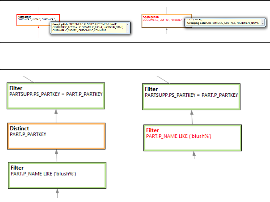
Table 1: Hint: GROUPING_SIMPLIFICATION
Before After
Table 2: Hint: GROUPING_REMOVAL
Before After
Related Information
HINT Details
5.5.7.3 Changing Operator Order
You can use hints to change the order of operators during plan generation.
By examining the plan, you can apply dierent hints to change the operator order as needed. By using
NO_<hint>, the operators can be disabled to produce the opposite eect. For a full list of available hints, see
HINT Details in the SAP HANA SQL and System Views Reference.
SAP HANA Performance Guide for Developers
SQL Query Performance
P U B L I C 127
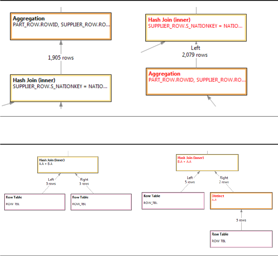
Table 3: Hint: AGGR_THRU_JOIN
Before After
Table 4: Hint: PREAGGR_BEFORE_JOIN
Before After
128 P U B L I C
SAP HANA Performance Guide for Developers
SQL Query Performance
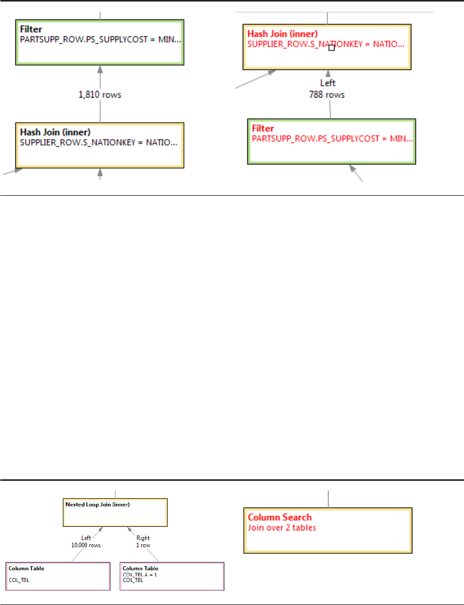
Table 5: Hint: FILTER_THRU_JOIN
Before After
Related Information
HINT Details
5.5.7.4 Choosing Preferred Algorithms
You can use hints to select preferred algorithms for execution (column engine versus row engine).
By using NO_<hint>, they can be disabled to produce the opposite eect. For a full list of available hints, see
HINT Details in the SAP HANA SQL and System Views Reference.
Table 6: Hint: CS_JOIN
Before After
SAP HANA Performance Guide for Developers
SQL Query Performance
P U B L I C 129
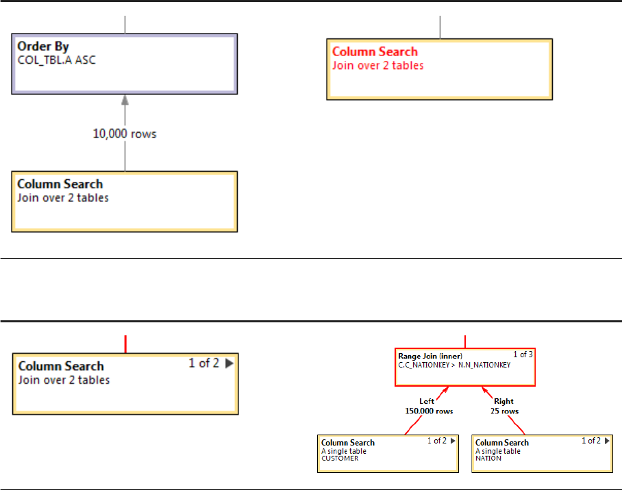
Table 7: Hint: CS_ORDERBY
Before After
Table 8: Hint: RANGE_JOIN
Before After
Related Information
HINT Details
5.5.7.5 Using ALTER SYSTEM to Pin Hints to Problematic
Queries
A hint table can be used to persist the binding between a query and its hints.
If you want to persist the binding between a query and its hints or you are unable to append hints to a query
during runtime (that is, for application-generated queries), a hint table can be used. For a full list of available
hints, see HINT Details in the SAP HANA SQL and System Views Reference.
130
P U B L I C
SAP HANA Performance Guide for Developers
SQL Query Performance

Related Information
HINT Details
5.5.8 Additional Recommendations
These specic recommendations have been derived from performance testing.
IFNULL (WHERE) (Workaround)
Avoid IFNULL in the WHERE clause by rewriting it:
Problematic
ifnull(jobReq.IS_DELETED, '0') = '0'
Sample Code
SELECT
MAX(application_date) as last_applied_date
FROM PERFSANITY_TEST.RCM_APPLICATION application,
PERFSANITY_TEST.RCM_JOB_REQ jobReq
WHERE application.JOB_REQ_ID = jobReq.JOB_REQ_ID
AND ifnull(jobReq.IS_DELETED, '0') = '0'
and application.status in (0, 1, 2, 3)
AND application.CANDIDATE_ID = ?
Recommended
(jobReq.IS_DELETED = '0' OR jobReq.IS_DELETED is null)
The example query improved from 121 milliseconds to 10 milliseconds.
IFNULL (SELECT) (Workaround)
Avoid IFNULL in the SELECT clause by rewriting it:
Problematic
ifnull(userSelectedLocale.job_title, defaultLocale.job_title) job_title
Recommended
SAP HANA Performance Guide for Developers
SQL Query Performance
P U B L I C 131

case userSelectedLocale.job_title when null then defaultLocale.job_title
else userSelectedLocale.job_title end job_title,
Sample Code
SELECT
jobreq.job_req_id,
case userSelectedLocale.job_title
when null then defaultLocale.job_title
else userSelectedLocale.job_title end job_title,
case userSelectedLocale.external_title
when null then defaultLocale.external_title
else userSelectedLocale.external_title end external_title
FROM PERFSANITY_TEST.RCM_JOB_REQ_LOCAL defaultLocale
The example query improved from 40 milliseconds to 20 milliseconds.
CONTAINS Versus LIKE
Replace LIKE <value> searches with CONTAINS:
Problematic
lower(u.USERS_SYS_LASTNAME) like ?
Recommended
CONTAINS(u.USERS_SYS_LASTNAME, ?)
Sample Code
SELECT * FROM ( SELECT u.users_sys_id, u.users_sys_username, ...
FROM PERFSANITY_TEST.USERS_SYSINFO u
WHERE CONTAINS( (u.USERS_SYS_LASTNAME,
u.USERS_SYS_FIRSTNAME,
u.USERS_SYS_MI,
u.USERS_SYS_NICKNAME), ?)
AND u.users_sys_valid = ?
ORDER BY lower(u.users_sys_FIRSTNAME) asc NULLS LAST) LIMIT ? OFFSET ?
The example query improved from 180 milliseconds to 14 milliseconds.
132
P U B L I C
SAP HANA Performance Guide for Developers
SQL Query Performance

NULLS FIRST on Non-Null Columns (Workaround)
Avoid NULLS FIRST or NULLS LAST on a non-null column:
Problematic
SELECT * FROM ( SELECT
jobInstance.instance_id,
jobInstance.status,
jobInstance.error_code,
jobInstance.submit_date,
jobRequest.job_name,
jobInstance.request_id,
jobRequest.job_type,
jobInstance.job_execution_id,
...
FROM PERFSANITY_TEST.JOB_INSTANCE jobInstance
LEFT JOIN PERFSANITY_TEST.JOB_REQUEST jobRequest ON
jobInstance.request_id=jobRequest.request_id
ORDER BY jobInstance.submit_date desc NULLS FIRST) LIMIT ?
Recommended
...
ORDER BY jobInstance.submit_date desc) LIMIT ?
The workaround can be applied without aecting the result if the column being sorted (in this case,
jobInstance.submit_date) does not contain any NULL values. In the example query, this condition was
met due to the following:
● The submit_date column in the JOB_INSTANCE table was dened as NOT NULL.
● The JOB_INSTANCE table was the left table in the LEFT JOIN.
The example query improved from 120 milliseconds to 15 milliseconds.
Nested Subselects with Outer Joins in FROM
Consider applying inlining to queries that show the following pattern:
SELECT ...
FROM (SUBSELECT A)
RIGHT OUTER JOIN (SUBSELECT B)
LEFT OUTER JOIN (SUBSELECT C)
LEFT OUTER JOIN (SUBSELECT D)
WHERE ...
Manually inlining the subselects into the outer SELECT can lead to signicant performance improvements
(from 1.0 seconds to 250 milliseconds in an example query, where some of the subselects were not yet inlined).
However, inlining needs to be done carefully to preserve the same semantics, particularly when combining
inner and outer joins.
SAP HANA Performance Guide for Developers
SQL Query Performance
P U B L I C 133
6 SQLScript Performance Guidelines
SQLScript allows data-intensive application logic to be embedded into the database. Conceptually SQLScript is
related to stored procedures as dened in the SQL standard, but SQLScript is designed to provide superior
optimization capabilities. These are key to avoiding massive data copies to the application server and to
leveraging the sophisticated parallel execution strategies of the SAP HANA database.
SQLScript should be used in cases where other modeling constructs of SAP HANA are not sucient.
Related Information
Calling Procedures [page 134]
Working with Tables and Table Variables [page 138]
Blocking Statement Inlining with the NO_INLINE Hint [page 150]
Skipping Expensive Queries [page 151]
Using Dynamic SQL with SQLScript [page 152]
Simplifying Application Coding with Parallel Operators [page 154]
Replacing Row-Based Calculations with Set-Based Calculations [page 162]
Avoiding Busy Waiting [page 165]
Best Practices for Using SQLScript [page 166]
6.1 Calling Procedures
By using parameters correctly when you call procedures, you not only make your code more robust and
readable, but also easier to parse and therefore faster to execute.
For better performance, SAP recommends that you use parameterized call statements:
● A parameterized query compiles once only, therefore reducing the compile time.
● A stored query string in the SQL plan cache is more generic and a precompiled query plan can be reused
for the same procedure call with dierent input parameters.
● When query parameters are not used in the call statement, the system triggers a new query plan
generation.
Related Information
Passing Named Parameters [page 135]
134
P U B L I C
SAP HANA Performance Guide for Developers
SQLScript Performance Guidelines

Changing the Container Signature [page 136]
Accessing and Assigning Variable Values [page 136]
Assigning Scalar Variables [page 138]
6.1.1 Passing Named Parameters
When you call a procedure, you can pass named parameters. Named parameters are recommended because
they improve the readability of the code and make the purpose of the parameters clear. They also provide
exibility because the order of the parameters in the call statement does not need to match the order in the
procedure signature.
You can pass named parameters by using the token =>.
For example, two ways in which the same procedure can be called are shown below, rstly without and
secondly with named parameters:
Without Named Parameters
DO (...)
BEGIN
...
CALL INNER_PROC (:tab,
:f,
:sd,
:es,
c_sum );
...
END;
With Named Parameters
DO (...)
BEGIN
...
CALL INNER_PROC ( cust_list => :tab,
filter_str => :f,
start_date => :sd,
end_date => :ed
cumulative_sum => c_sum );
...
END;
In the rst example, the order of the parameters must be the same as in the procedure signature. In the
second, however, this order can be ignored. Note that this makes procedure calls more robust with respect to
changes to the container signature.
SAP HANA Performance Guide for Developers
SQLScript Performance Guidelines
P U B L I C 135

6.1.2 Changing the Container Signature
By using named parameters, you make your procedure calls more exible and robust with respect to changes
to the container signature.
The examples below show how changes to container signatures can aect procedure calls:
Initial Container Signature
CREATE PROCEDURE P ( IN iv_tab TTYPE,
OUT ov_tab TTYPE
)
AS
BEGIN
...
END;
CALL P (iv_tab => inputTab, ov_tab => ?);
CALL P (inputTab, ?);
Changed Container Signa
ture
CREATE PROCEDURE P ( IN iv_tab TTYPE,
OUT ov_tab TTYPE,
IN var INTEGER DEFAULT NULL,
IN iv_tab2 DUMMY DEFAULT DUMMY,
IN iv_tab3 TTYPE DEFAULT EMPTY
)
AS
BEGIN
...
END;
CALL P (iv_tab => inputTab, ov_tab => ?);
CALL P (inputTab, ?);
● The rst example shows the initial container signature and two procedure calls created for it, rstly with
and secondly without named parameters.
● In the second example, the container signature includes three additional parameters with default values:
○ Parameters with default values can be omitted in procedure calls with named parameters. The rst
procedure call is therefore not aected by the changes.
○ Parameters with default values cannot be omitted in procedure calls without named parameters. The
second procedure call is therefore aected by the changes, even though the initial parameter order has
not changed.
6.1.3 Accessing and Assigning Variable Values
By using a colon (:) together with variables, you can make your code more readable as well as indicate to the
parser whether a variable value should be read or written.
To access a value from a variable (that is, to read) use the colon. To assign a value to a variable (that is, to
write), do not use a colon. By observing these rules, you not only make your code more readable but also easier
to parse.
136
P U B L I C
SAP HANA Performance Guide for Developers
SQLScript Performance Guidelines

Consider the following examples:
Problematic
DO (OUT tab TABLE( a INT, b INT) => ?)
BEGIN
DECLARE c INT = 10;
DECLARE b INT = 20;
...
tab = SELECT A AS A, b AS B FROM T WHERE C=c;
END;
Recommended
DO (OUT tab TABLE( a INT, b INT) => ?)
BEGIN
DECLARE c INT = 10;
DECLARE b INT = 20;
...
tab = SELECT A AS A, :b AS B FROM T WHERE C=:c;
END;
● In the rst example above, it is not clear to the parser how to handle b and c. The column c is unknown and
b is interpreted as a column.
● In the second example, the colon indicates that it is the values of the two declared variables b and c that
need to be read.
Problematic
DO (...)
BEGIN
...
CALL INNER_PROC (tab, f, sd, ed, c_sum );
...
END;
Recommended
DO (...)
BEGIN
...
CALL INNER_PROC (:tab, :f, :sd, :ed, c_sum);
...
END;
● In the rst example, it is not clear to the parser whether values should be read from or written to the
variables tab, f, sd, ed, and c_sum.
● In the second example, the colon indicates that the values should be read from the tab, f, sd, and ed
variables. The variable c_sum, however, should be assigned a value.
SAP HANA Performance Guide for Developers
SQLScript Performance Guidelines
P U B L I C 137

6.1.4 Assigning Scalar Variables
Scalar variables can be assigned using the assignment operator =. Note that it is the same way as for table
variables.
For example:
DO (OUT tab TABLE( a int, b int ) => ?)
BEGIN
DECLARE c INT = 10;
DECLARE b INT = 20;
...
tab = SELECT * FROM T;
END;
6.2 Working with Tables and Table Variables
The recommended programming patterns allow you to eciently access and manipulate tables and table
variables.
Related Information
Checking Whether a Table or Table Variable is Empty [page 138]
Determining the Size of a Table Variable or Table [page 140]
Accessing a Specic Table Cell [page 141]
Searching for Key-Value Pairs in Table Variables [page 142]
Avoiding the No Data Found Exception [page 144]
Inserting Table Variables into Other Table Variables [page 144]
Inserting Records into Table Variables [page 145]
Updating Individual Records in Table Variables [page 147]
Deleting Individual Records in Table Variables [page 148]
6.2.1 Checking Whether a Table or Table Variable is Empty
The recommended way to check whether a table variable or table is empty is to use the predicate IS_EMPTY.
Compare the following examples:
Problematic: SELECT COUNT(*)
138 P U B L I C
SAP HANA Performance Guide for Developers
SQLScript Performance Guidelines

CREATE PROCEDURE P (
IN iv_tab TABLE(…),…)
AS
BEGIN
DECLARE size INTEGER;
SELECT COUNT(*) INTO size
FROM :iv_tab;
IF :size <= 0 THEN
RETURN;
END IF;
...
END;
Problematic: CARDINALITY
CREATE PROCEDURE P (
IN iv_tab TABLE(…),…)
AS
BEGIN
DECLARE size INTEGER;
size =
CARDINALITY(
ARRAY_AGG(:iv_tab.A)
);
IF :size <= 0 THEN
RETURN;
END IF;
...
END;
Recommended: IS_EMPTY
CREATE PROCEDURE P (
IN iv_tab TABLE(…),…)
AS
BEGIN
IF IS_EMPTY(:iv_tab) THEN
RETURN;
END IF;
...
END;
● In the rst example, SELECT COUNT is used determine the size of the table variable. This approach is not
recommended because it involves a select query, which is expensive.
● The second example, which uses the CARDINALITY function, is faster than the rst example because it
does not involve a query. However, it requires the data to be copied into an array, which has an impact on
performance.
● The recommended method is to use IS_EMPTY, which involves one direct operation on the table variable.
Note that another recommended option is to use RECORD_COUNT.
SAP HANA Performance Guide for Developers
SQLScript Performance Guidelines
P U B L I C 139

6.2.2 Determining the Size of a Table Variable or Table
For the best performance, you should use RECORD_COUNT rather than COUNT or CARDINALITY.
RECORD_COUNT is the fastest option. It simply takes the name of the table or table variable as the argument
and returns the number of records.
COUNT and CARDINALITY are both slower and have a greater impact on performance (see the previous topic).
The two examples below show the use of CARDINALITY and RECORD_COUNT, where the derived size of the
table variable is used to construct a loop:
Problematic: CARDINALITY
DO (IN inTab TABLE(i int) => TAB,...)
BEGIN
DECLARE i int;
DECLARE v nvarchar(200);
FOR i IN 1 .. CARDINALITY(ARRAY_AGG(:inTab.I))
DO
v = :t.col_a[:i];
...
END FOR;
END;
Recommended: RECORD_COUNT
DO (IN inTab TABLE(i int) => TAB,...)
BEGIN
DECLARE i int;
DECLARE v nvarchar(200);
FOR i IN 1 .. record_count(:inTab)
DO
v = :t.col_a[:i];
...
END FOR;
END;
140 P U B L I C
SAP HANA Performance Guide for Developers
SQLScript Performance Guidelines

6.2.3 Accessing a Specic Table Cell
To access a specic cell of a table variable, use index-based access rather than a select query or an array. This
is faster and has a lower impact on performance.
Reading a Value
The examples below read the values from the rst row of the two columns A and B. Note that for read access a
colon (:) is needed before the table variable:
Problematic: Query
CREATE PROCEDURE P (
IN iv_tab TABLE(A INT, B NVARCHAR(28)),…)
AS
BEGIN
DECLARE var_a INT;
DECLARE var_b NVARCHAR(28);
SELECT TOP 1 A, B INTO var_a, var_b
FROM :iv_tab;
...
END;
Recommended: Index-Based Cell Access
CREATE PROCEDURE P (
IN iv_tab TABLE(A INT, B NVARCHAR(28)),…)
AS
BEGIN
DECLARE var_a INT;
DECLARE var_b NVARCHAR(28);
var_a = :iv_tab.A[1];
var_b = :iv_tab.B[1];
...
END;
● The rst example shows the slower option, where a SELECT INTO query is used to return the rst entry
(TOP 1) from columns A and B.
● The second example uses index-based access to read the values from the rst row of the two columns A
and B.
Writing a Value
The examples below write a value to the second row of column A:
Problematic: Array
SAP HANA Performance Guide for Developers
SQLScript Performance Guidelines
P U B L I C 141

CREATE PROCEDURE P (
IN iv_tab TABLE(A INT, B NVARCHAR(28)),…)
AS
BEGIN
DECLARE a_arr INT ARRAY;
DECLARE b_arr NVARCHAR(28) ARRAY;
a_arr = ARRAY_AGG(:iv_tab.A);
b_arr = ARRAY_AGG(:iv_tab.B);
a_arr[2] = 5;
iv_tab = UNNEST(:a_arr, :b_arr) AS (A,B);
...
END;
Recommended: Index-Based Cell Access
CREATE PROCEDURE P (
IN iv_tab TABLE(A INT, B NVARCHAR(28)),…)
AS
BEGIN
iv_tab.A[2] = 5;
...
END;
● The slower option in the rst example involves converting the two columns A and B of the table variable
iv_tab into arrays, then writing the new value 5 to the second cell in array a_arr. The two arrays are then
converted back into a table using the UNNEST function and assigned to the table variable iv_tab.
● The second example shows how index-based access can be used to directly access the second row of
column A in the iv_tab table variable and insert the value 5.
6.2.4 Searching for Key-Value Pairs in Table Variables
The SEARCH operator provides the most ecient way to search table variables by key-value pairs. It returns
the position of the rst record that matches the search criteria, or NULL if there are no matches.
The syntax is as follows:
position = <tabvar>.SEARCH((<column_list>), (<value_list>) [, <start_position>])
For example, you have the following table named LT1:
Key 1
Key 2 Val 1
A 1 V11
E 5 V12
M 3 V15
142 P U B L I C
SAP HANA Performance Guide for Developers
SQLScript Performance Guidelines

You now run the following code:
DO (IN lt1 TABLE
(KEY1 NVARCHAR(1), Key2 INT, Val1 NVARCHAR(3)) => tab,...)
BEGIN
DECLARE pos INT;
DECLARE val LIKE :lt1.Val1;
IF :lt1.SEARCH((key1,key2), ('I',3)) IS NULL THEN
:lt1.insert(('I',3,'X'));
END IF;
pos = :lt1.SEARCH((key1,key2), ('M',3));
:lt1.delete(:pos);
val = :lt1.val1[:lt1.SEARCH((Key1,Key2),('E',5))];
...
END;
The rst SEARCH operation is used to determine whether
the table already contains the key-value pair
('I',3) so
that, if not, the record ('I',3,'X') can be inserted.
Since there is no record that matches, the new record is in
serted:
Key 1
Key 2 Val 1
A 1 V11
E 5 V12
M 3 V15
I 3 X
The second SEARCH operation is used to determine
whether the key-value pair
('M',3) exists. Since the value
of pos (not NULL) conrms that it does, the record can be
deleted:
Key 1
Key 2 Val 1
A 1 V11
E 5 V12
M 3 V15
I 3 X
The third search operation retrieves the position of the value
pair
('E',5), which is then used to assign the value of
val1 to val (the value of val is then V12):
Key 1 Key 2 Val 1
A 1 V11
E 5 V12
I 3 X
SAP HANA Performance Guide for Developers
SQLScript Performance Guidelines
P U B L I C 143

6.2.5 Avoiding the No Data Found Exception
The SELECT INTO statement does not accept an empty result set. To avoid a no data found exception being
thrown when a result set is empty, this condition should be handled by either an exit handler, an emptiness
check, or by assigning default values.
For example, the following query is run, but the result set is empty:
SELECT EID INTO ex_id FROM :tab;
SAP DBTech JDBC: [1299]: no data found: [1299] "SESSION28480"."GET_ID": line 14
col 4 (at pos 368):
[1299] (range 3) no data found exception: no data found
The examples below show how the three options mentioned above can be applied:
Exit Handler
Emptiness Check Default Value
DECLARE EXIT HANDLER FOR
SQL_ERROR_CODE 1299
BEGIN
ex_id = NULL;
END;
SELECT EID INTO ex_id
FROM :tab;
IF is_empty(:tab) THEN
ex_id = NULL;
ELSE
ex_id
= :tab.EID[1];
END IF;
SELECT EID INTO ex_id
DEFAULT NULL
FROM :tab;
● In the rst example, an exit handler is dened specically for the SQL error code 1299. If the result set is
empty, it assigns the value NULL to the target variable ex_id.
● In the second example, the IS_EMPTY predicate is used to check whether the result set is empty. If this is
the case, the target variable ex_id is assigned the value NULL.
● The third example makes uses of the DEFAULT values feature supported by the SELECT INTO statement,
which has the following syntax:
SELECT <select_list> INTO <var_name_list> [DEFAULT <scalar_expr_list>]
<from_clause>
6.2.6 Inserting Table Variables into Other Table Variables
The most ecient way to insert the content of one table variable into another is to use the INSERT operator.
The insertion is done in one operation and does not involve using an SQL query. An alternative approach using
the UNION operator has a higher performance cost.
The following two examples compare the use of the UNION and INSERT operators:
Problematic: Query
144 P U B L I C
SAP HANA Performance Guide for Developers
SQLScript Performance Guidelines

DO (OUT ret_tab TABLE(col_a nvarchar(200))=>?)
BEGIN
DECLARE i int;
DECLARE varb nvarchar(200);
...
FOR i IN 1 .. record_count(:t) DO
CALL p (:varb, out_tab);
ret_tab = SELECT COL_A FROM :out_tab
UNION SELECT COL_A FROM :ret_tab;
...
END FOR;
END;
Recommended: INSERT
DO (OUT ret_tab TABLE(col_a nvarchar(200))=>?)
BEGIN
DECLARE i int;
DECLARE varb nvarchar(200);
...
FOR i IN 1 .. record_count(:t) DO
CALL p (:varb, out_tab);
:ret_tab.insert(:out_tab);
...
END FOR;
END;
The examples combine col_a from the table variable out_tab with col_a in the table variable ret_tab:
● In the rst example, the UNION operator is used to combine the result sets of two select queries. This is a
costly operation in terms of performance.
● The syntax used for the INSERT operation (second example) is as follows:
:<target_table_var>[.(<column_list>)].INSERT(:<source_table_var>[,
<position>])
○ A position is not specied in the example, so the values are simply appended at the end. Similarly, no
columns are specied, so all columns are inserted. In this example, there is only the one column,
col_a.
○ The souce and target columns must be of the same data type, in this case it is NVARCHAR.
6.2.7 Inserting Records into Table Variables
For scenarios requiring individual data records to be inserted at the end of a table variable, the recommended
way is to use the INSERT operator. The insertion is done in one operation and is faster and more ecient than
the alternative approaches using arrays or index-based cell access.
The three examples below compare the ways in which 10 rows can be inserted at the end of a table variable
using index-based array access, index-based cell access, and the INSERT operator:
SAP HANA Performance Guide for Developers
SQLScript Performance Guidelines
P U B L I C 145

Problematic: Array
CREATE PROCEDURE P (
IN iv_tab TABLE(A INT, B NVARCHAR(28),…),
…)
AS
BEGIN
DECLARE a_arr INT ARRAY;
DECLARE b_arr NVARCHAR(28) ARRAY;
DECLARE c_arr NVARCHAR(28) ARRAY;
DECLARE sizeTab,i BIGINT;
a_arr = ARRAY_AGG(:iv_tab.A);
b_arr = ARRAY_AGG(:iv_tab.B);
c_arr = ARRAY_AGG(:iv_tab.C);
sizeTab = CARDINALITY(:a_arr);
FOR i IN 1 .. 10 DO
A_ARR[:sizeTab+i] = 1;
B_ARR[:sizeTab+i] = 'ONE';
C_ARR[:sizeTab+i] = 'EINS';
END FOR;
iv_tab = UNNEST(:a_arr,:b_arr,:c_arr)
AS (A,B,C);
END;
Problematic: Index-Based Cell Access
CREATE PROCEDURE P (
IN iv_tab TABLE(A INT, B NVARCHAR(28),… ))
…)
AS
BEGIN
DECLARE sizeTab,i BIGINT;
sizeTab = RECORD_COUNT(:iv_tab);
FOR i IN 1 .. 10 DO
iv_tab.A[:sizeTab+i] = 1;
iv_tab.B[:sizeTab+i] = 'ONE';
iv_tab.C[:sizeTab+i] = 'EINS';
END FOR;
END;
Recommended: INSERT
146 P U B L I C
SAP HANA Performance Guide for Developers
SQLScript Performance Guidelines

CREATE PROCEDURE P (
IN iv_tab TABLE(A INT, B NVARCHAR(28),…),
…)
AS
BEGIN
DECLARE i BIGINT;
FOR i IN 1 .. 10 DO
:iv_tab.INSERT(( 1,'ONE','EINS'));
END FOR;
END;
● The rst example has the highest impact on performance:
○ Each column of the table variable needs to be converted into an array.
○ The CARDINALITY function needs to be executed to determine the size of the array.
○ The determined size is used within the loop to append the values at the end of each array.
○ UNNEST is used to convert the arrays back into a table variable.
● The second example is faster but still requires the following:
○ The size of the table variable is determined using RECORD_COUNT.
○ The determined size is used within the loop to append the values at the end of each column (see the
next topic for an example of how this could be improved).
● The third example uses INSERT, which is recommended for the following reasons:
○ It is not necessary to determine the size of the table variable. If a position is not given in the INSERT
statement, the new values are simply appended at the end of the table variable.
○ INSERT allows entire rows to be inserted. The syntax is as follows:
:<table_variable>.INSERT((<value1,…, <valueN), <index>)
6.2.8 Updating Individual Records in Table Variables
It is more ecient to update all applicable values in a table row in one operation, for example, using the
UPDATE operator or index-based row access, rather than individual table cells (index-based cell access).
The two examples below show how a record at a specic position can be updated:
Problematic: Index-Based Cell Access
SAP HANA Performance Guide for Developers
SQLScript Performance Guidelines
P U B L I C 147

CREATE PROCEDURE P (
IN iv_tab TABLE(A INT, B NVARCHAR(28)…),…)
AS
BEGIN
iv_tab.A[42] = 1;
iv_tab.B[42] = 'ONE';
iv_tab.C[42] = 'EINS';
...
END;
Recommended: UPDATE
CREATE PROCEDURE P (
IN iv_tab TABLE(A INT, B NVARCHAR(28)),…)
AS
BEGIN
iv_tab[42] = (1, 'ONE', 'EINS');
iv_tab.update((1, 'ONE', 'EINS'),42);
...
END;
● In the rst example, index-based cell access is used to assign new values to each column separately.
● In the second example, the entire row is updated in a single operation. There are two equivalent syntax
options:
○ :<table_variable>.UPDATE((<value1>,…, <valuen>), <index>)
○ <table_variable>[<index>] = (<value1>,…, <valuen>)
6.2.9 Deleting Individual Records in Table Variables
The DELETE operator is the most ecient way of deleting records from a table variable. It allows you to delete
single records, a range of records, or selected records.
The two examples below show how the last record in the table variable can be deleted:
Problematic: Query
148 P U B L I C
SAP HANA Performance Guide for Developers
SQLScript Performance Guidelines

CREATE PROCEDURE P (
IN iv_tab TABLE(A INT, B NVARCHAR(28),... ))
AS
BEGIN
DECLARE rc BIGINT = RECORD_COUNT(:iv_tab);
...
iv_tab_temp = SELECT
ROW_NUMBER() OVER() AS ROW_NO,
it.*
FROM :iv_tab AS it;
iv_tab = SELECT itt.A, itt.B, itt.C
FROM :iv_tab_temp as itt
WHERE row_no <> :rc;
...
END;
Recommended: DELETE
CREATE PROCEDURE P (
IN iv_tab TABLE(A INT, B NVARCHAR(28), ...))
AS
BEGIN
:iv_tab.delete(RECORD_COUNT(:iv_tab));
:iv_tab.delete(42..100);
:iv_tab.delete();
...
END;
● The rst example uses queries:
○ The size of the table variable is determined using RECORD_COUNT.
○ A SELECT query copies the entire contents of the table variable iv_tab to a temporary table
iv_tab_temp. The ROW_NUMBER function is used to number the rows within the result set.
○ A SELECT query copies all rows except the last row (determined by RECORD_COUNT) from the
temporary table back to the table variable iv_tab.
● The second example uses the DELETE operator:
○ The size of the table variable is determined using RECORD_COUNT.
○ The syntax of the DELETE operator is as follows:
:<table_variable>.DELETE(<index>)
The index of the last row has been determined by RECORD_COUNT.
Note that if an index is not specied, all rows are deleted. For example:
:iv_tabl:delete();
SAP HANA Performance Guide for Developers
SQLScript Performance Guidelines
P U B L I C 149

Other syntax options supported by the DELETE operator:
○ Delete a block:
:<table_variable>.DELETE(<from_index>..<to_index>)
○ Delete a selection:
:<table_variable>.DELETE(<array_of_integers>)
6.3 Blocking Statement Inlining with the NO_INLINE Hint
The SQLScript compiler combines inline (that is, dependent) statements if possible to optimize the code.
There might be cases, however, where the combined statements do not result in an optimal plan. This therefore
aects performance when the statement is executed.
To prevent a statement from being combined with other statements, you can use the NO_INLINE hint. It needs
to be placed at the end of the SELECT statement.
Note
Use the NO_INLINE hint carefully, since it directly impacts performance. Separate statements are generally
more expensive.
The examples below show a scenario where the use of NO_HINT is benecial:
Problematic
DO (OUT tab2 TABLE (c int) => ?)
BEGIN
tab = SELECT A, B, C
FROM T WHERE A = 1;
tab2 = SELECT C FROM :tab WHERE C = 0;
END;
Combined query
WITH "_SYS_TAB_2" AS (SELECT A, B, C
FROM T WHERE A = 1) SELECT C FROM "_SYS_TAB_2"
WHERE C = 0
Recommended
DO (OUT tab2 TABLE (c int) => ?)
BEGIN
tab = SELECT A, B, C
FROM T WHERE A = 1 WITH HINT(NO_INLINE);
tab2 = SELECT C FROM :tab WHERE C = 0;
END;
150 P U B L I C
SAP HANA Performance Guide for Developers
SQLScript Performance Guidelines

tab
SELECT A, B, C FROM T
WHERE A = 1 WITH HINT ( NO_INLINE )
tab2
SELECT C FROM ( SELECT A, B, C FROM
"MY_SCHEMA"."_SYS_CE_TAB_2_SYS_SS_CE_DO_TMP_CALL_popid_3_57C4F795270F49E4E100000
00A445C43_283" )_SYS_SS_VAR_TAB_2
WHERE "C" = 0
● In the rst example, the resulting code of the combined query indicates that the SQLScript optimizer was
not able to determine the best way to combine the two statements.
● In the second example, the table variable assignments show that each statement was executed separately,
due to the addition of WITH HINT(NO_INLINE) in the rst statement.
6.4 Skipping Expensive Queries
You can skip a query within a procedure by using a constant predicate that evaluates to false. Skipping an
expensive query is an eective measure for improving performance.
The three examples below show the ways in which an expensive query can be handled within a procedure:
Problematic
CREATE PROCEDURE get_product_by_filter(IN im_input_string VARCHAR(5000))
AS
BEGIN
step1 = SELECT * FROM VIEW1;
step2 = SELECT * FROM EXPENSIVE_FUNC(:im_input_string);
res = SELECT * FROM :step1 UNION ALL
SELECT * FROM :step2;
...
END;
Recommended
CREATE PROCEDURE get_product_by_filter(IN im_input_string VARCHAR(5000))
AS
BEGIN
step1 = SELECT * FROM VIEW1;
step2 = SELECT * FROM EXPENSIVE_FUNC(:im_input_string) WHERE :im_input_string
NOT IN ('foo', 'bar');
res = SELECT * FROM :step1 UNION ALL
SELECT * FROM :step2;
...
END;
SAP HANA Performance Guide for Developers
SQLScript Performance Guidelines
P U B L I C 151

Recommended
CREATE PROCEDURE get_product_by_filter(IN im_input_string VARCHAR(5000))
AS
BEGIN
DECLARE skip_query SMALLINT := 0;
IF (:im_input_string IN ('foo', 'bar') ) THEN
skip_query = 1;
END IF;
step1 = SELECT * FROM VIEW1;
step2 = SELECT * FROM EXPENSIVE_FUNC(:im_input_string) WHERE :skip_query = 1;
res = SELECT * FROM :step1 UNION ALL
SELECT * FROM :step2;
...
END;
● In the rst example, the expensive query (shown in bold) is always executed.
● In the second example, a condition is applied in the WHERE clause of the expensive query. When the
condition evaluates to false, the query will not be executed.
● In the third example, the condition (here skip_query) is declared using an IF clause. As above, it is applied
in the WHERE clause of the expensive query. When the condition evaluates to false, this will lead to the
query being pruned and as a result not executed.
6.5 Using Dynamic SQL with SQLScript
In general, it is not recommended to use dynamic SQL in SQLScript procedures, since it can have a negative
impact on performance and security.
Executing dynamic SQL is slow due to the compile-time checks and query optimizations that need to be
performed each time the procedure is called. Also, the opportunities for optimizations are limited, and the
statement is potentially recompiled every time it is executed.
In addition, constructing SQL statements without proper checks of the variables used can create a security
vulnerability, for example, SQL injection.
To use dynamic SQL in an ecient and secure manner, you can use input and output parameters.
Related Information
Using Input and Output Parameters [page 153]
152
P U B L I C
SAP HANA Performance Guide for Developers
SQLScript Performance Guidelines

6.5.1 Using Input and Output Parameters
The INTO and USING clauses of the EXECUTE IMMEDIATE and EXEC statements provide additional support for
parameterizing dynamic SQL. The INTO clause can be used to assign the result sets or output parameters of a
query to scalar or table variables.
The two examples below compare a string built using dynamic SQL and a parameterized version of the same
code:
Problematic: Building the String
DO (IN I INT => ?, IN J NVARCHAR(28)=> ? )
BEGIN
DECLARE TNAME nvarchar(32) = 'MYTAB’;
DECLARE CNAME nvarchar(32) = 'AGE';
EXECUTE IMMEDIATE
'SELECT MAX('|| :CNAME ||') AS MAX, NAME FROM '
|| :TNAME ||
' WHERE A = ' ||:I ||' OR B='''||:J||'''GROUP BY name';
END;
SELECT MAX(AGE) AS MAX,NAME FROM MYTAB WHERE A=1 OR B='ONE'
SELECT MAX(AGE) AS MAX,NAME FROM MYTAB WHERE A=2 OR B='TWO'
Recommended: With Parameters
DO (IN I INT => 1, IN J NVARCHAR(28)=> 'ONE')
OUT K TABLE ( MAX INT, NAME NVARCHAR(256)) => ?)
BEGIN
DECLARE TNAME nvarchar(32) = 'MYTAB';
DECLARE CNAME nvarchar(32) = 'AGE';
EXECUTE IMMEDIATE
'SELECT MAX('|| :CNAME ||') AS MAX, NAME FROM '
|| :TNAME ||
' WHERE A = ? OR B = ? group by NAME '
INTO K
USING :I,:J;
END;
SELECT MAX(AGE) AS MAX,NAME FROM MYTAB WHERE A=? OR B=?
●
In the rst example, the concatenated SQL strings contain the input values because parameters were not
used in the select statement. The resulting SQL string is stored in the plan cache. If the string is changed,
this will cause a conict with the plan cache.
● In the second example, the code is parameterized as follows:
○ The table variable K is dened as an output parameter. The INTO clause is used to assign the result set
to the table variable K. This allows it to be used in further processing.
○ The select statement is parameterized. The USING clause is used to pass in the values of the scalar
variables I and J. Although the input values are constants, the query is still parameterized.
○ The concatenated SQL string has a more generic form and will not cause the conicts seen above
when stored in the plan cache.
SAP HANA Performance Guide for Developers
SQLScript Performance Guidelines
P U B L I C 153

6.6 Simplifying Application Coding with Parallel Operators
Parallel operators allow sequential execution to be replaced with parallel execution. By identifying costly
sequential coding and using parallel operators in its place, you can signicantly improve performance. The
supported parallel operators are MAP_MERGE and MAP_REDUCE (a specialization of MAP_MERGE).
The targeted sequential coding patterns are those consisting of FOR loops, where operations are performed
separately on each row of a table, and UNION operators, which typically combine the results.
With the MAP_MERGE operator, a mapper function is applied to each row of a mapper table and the results
returned in an intermediate result table for each row. On completion, all intermediate results tables are
combined into a single table.
This form of parallel execution allows signicant performs gains:
● See the example in the Map Merge Operator topic below, which replaces sequential execution with parallel
execution. As a result, performance improved from 165 milliseconds to 29 milliseconds.
● See the Map Reduce Operator topic for a graphical illustration of the process.
Related Information
Map Merge Operator [page 154]
Map Reduce Operator [page 156]
6.6.1 Map Merge Operator
Description
The MAP_MERGE operator is used to apply each row of the input table to the mapper function and unite all
intermediate result tables. The purpose of the operator is to replace sequential FOR-loops and union patterns,
like in the example below, with a parallel operator.
Sample Code
DO (OUT ret_tab TABLE(col_a nvarchar(200))=>?)
BEGIN
DECLARE i int;
DECLARE varb nvarchar(200);
t = SELECT * FROM tab;
FOR i IN 1 .. record_count(:t) DO
varb = :t.col_a[:i];
CALL mapper(:varb, out_tab);
ret_tab = SELECT * FROM :out_tab
UNION SELECT * FROM :ret_tab;
END FOR;
154
P U B L I C
SAP HANA Performance Guide for Developers
SQLScript Performance Guidelines

END;
Note
The mapper procedure is a read-only procedure with only one output that is a tabular output.
Syntax
<table_variable> = MAP_MERGE(<table_or_table_variable>, <mapper_identifier>
(<table_or_table_variable>.<column_name> [ {,
<table_or_table_variable>.<column_name>} … ] [,
<param_list>])
<param_list> ::= <param> [{, <param>} …] <paramter> =
<table_or_table_variable>
| <string_literal> | <numeric_literal> |
<identifier>
The rst input of the MAP_MERGE operator is th mapper table <table_or_table_variable> . The mapper
table is a table or a table variable on which you want to iterate by rows. In the above example it would be table
variable t.
The second input is the mapper function <mapper_identifier> itself. The mapper function is a function you
want to have evaluated on each row of the mapper table <table_or_table_variable>. Currently, the
MAP_MERGE operator supports only table functions as <mapper_identifier>. This means that in the above
example you need to convert the mapper procedure into a table function.
You also have to pass the mapping argument <table_or_table_variable>.<column_Name> as an input of
the mapper function. Going back to the example above, this would be the value of the variable varb.
Example
As an example, let us rewrite the above example to leverage the parallel execution of the MAP_MERGE operator.
We need to transform the procedure into a table function, because MAP_MERGE only supports table functions
as <mapper_identifier>.
Sample Code
CREATE FUNCTION mapper (IN a nvarchar(200))
RETURNS TABLE (col_a nvarchar(200))
AS
BEGIN
ot = SELECT :a AS COL_A from dummy;
RETURN :ot;
END;
After transforming the mapper procedure into a function, we can now replace the whole FOR loop by the
MAP_MERGE operator.
SAP HANA Performance Guide for Developers
SQLScript Performance Guidelines
P U B L I C 155

Sequential FOR-Loop Version Parallel MAP_Merge Operator
DO (OUT ret_tab TABLE(col_a
nvarchar(200))=>?)
BEGIN
DECLARE i int;
DECLARE varb nvarchar(200);
t = SELECT * FROM tab;
FOR i IN 1 .. record_count(:t)
DO
varb = :t.col_a[:i];
CALL mapper(:varb,
out_tab);
ret_tab = SELECT *
FROM :out_tab
UNION SELECT *
FROM :ret_tab;
END FOR;
END;
DO (OUT ret_tab TABLE(col_a
nvarchar(200))=>?)
BEGIN
t = SELECT * FROM tab;
ret_tab = MAP_MERGE(:t,
mapper(:t.col_a));
END;
6.6.2 Map Reduce Operator
MAP_REDUCE is a programming model introduced by Google that allows easy development of scalable parallel
applications for processing big data on large clusters of commodity machines. The MAP_REDUCE operator is a
specialization of the MAP_MERGE operator.
Syntax
Code Syntax
MAP_REDUCE(<input table/table variable name>, <mapper specification>,
<reducer specification>)
<mapper spec> ::= <mapper TUDF>(<list of mapper parameters>) group by <list
of columns in the TUDF> as <ID>
<reducer spec> ::= <reduce TUDF>(<list of reducer TUDF parameters>)
| <reduce procedure>(<list of reducer procedure parameters>)
<mapper parameter> ::= <table/table variable name>.<column name> | <other
scalar parameter>
<reducer TUDF parameter> ::= <ID> | <ID>.<key column name> | <other scalar
parameter>
<reducer procedure parameter> ::= <reducer TUDF parameter> | <output table
parameter>
156
P U B L I C
SAP HANA Performance Guide for Developers
SQLScript Performance Guidelines

Example
We take as an example a table containing sentences with their IDs. If you want to count the number of
sentences that contain a certain character and the number of occurrences of each character in the table, you
can use the MAP_REDUCE operator in the following way:
Mapper Function
Sample Code
Mapper Function
create function mapper(in id int, in sentence varchar(5000))
returns table (id int, c varchar, freq int) as begin
using sqlscript_string as lib;
declare tv table(result varchar);
tv = lib:split_to_table(:sentence, ' ');
return select :id as id, result as c, count(result) as freq from :tv
group by result;
end;
Reducer Function
Sample Code
Reducer Function
create function reducer(in c varchar, in vals table(id int, freq int))
returns table (c varchar, stmt_freq int, total_freq int) as begin
return select :c as c, count(distinct(id)) as stmt_freq, sum(freq) as
total_freq from :vals;
end;
Sample Code
do begin
declare result table(c varchar, stmt_freq int, total_freq int);
result = MAP_REDUCE(tab, mapper(tab.id, tab.sentence) group by c as X,
reducer(X.c, X));
select * from :result order by c;
end;
The code above works in the following way:
1. The mapper TUDF processes each row of the input table and returns a table.
SAP HANA Performance Guide for Developers
SQLScript Performance Guidelines
P U B L I C 157
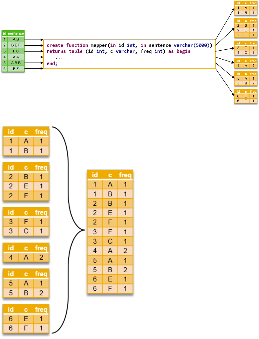
2. When all rows are processed by the mapper, the output tables of the mapper are aggregated into a single
big table (like MAP_MERGE).
3. The rows in the aggregated table are grouped by key columns.
158
P U B L I C
SAP HANA Performance Guide for Developers
SQLScript Performance Guidelines
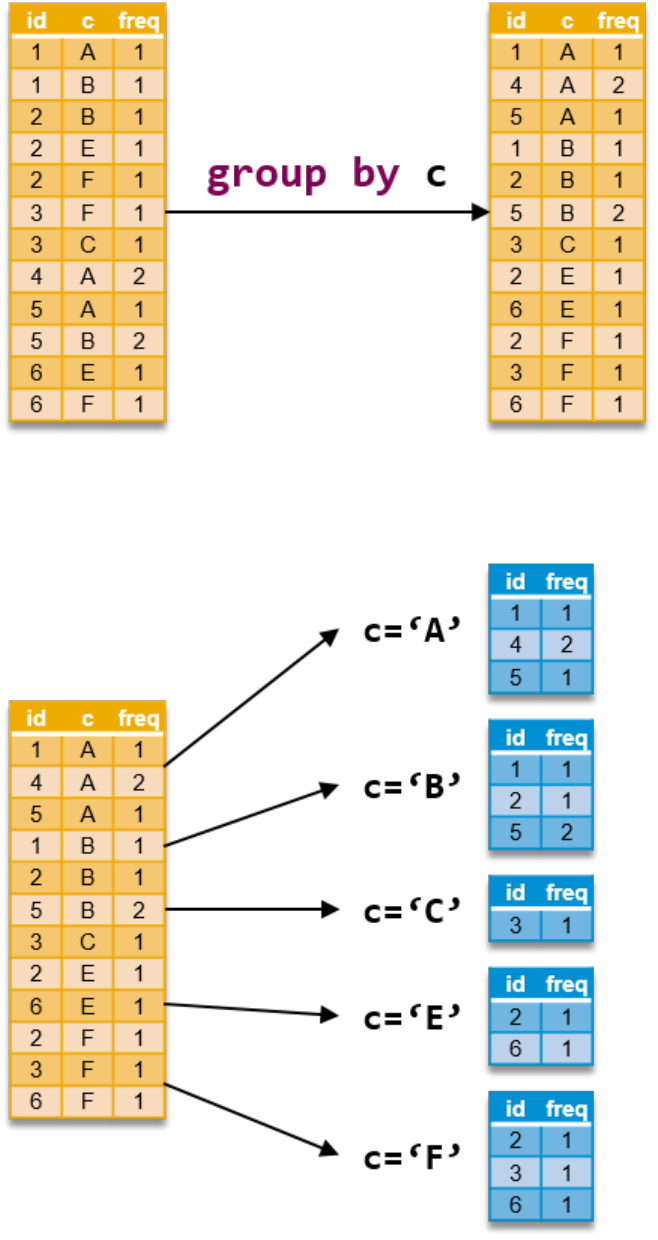
4. For each group, the key values are separated from the table. The grouped table without key columns is
called 'value table'. The order of the rest of columns is preserved. It is possible to have multiple key
columns. If the layout of the output table is table(a int, b varchar, c timestamp, d int) and
the key column is b and c, the layout of the value table is table(a int, d int).
5. The reducer TUDF (or procedure) processes each group and returns a table (or multiple tables).
SAP HANA Performance Guide for Developers
SQLScript Performance Guidelines
P U B L I C 159
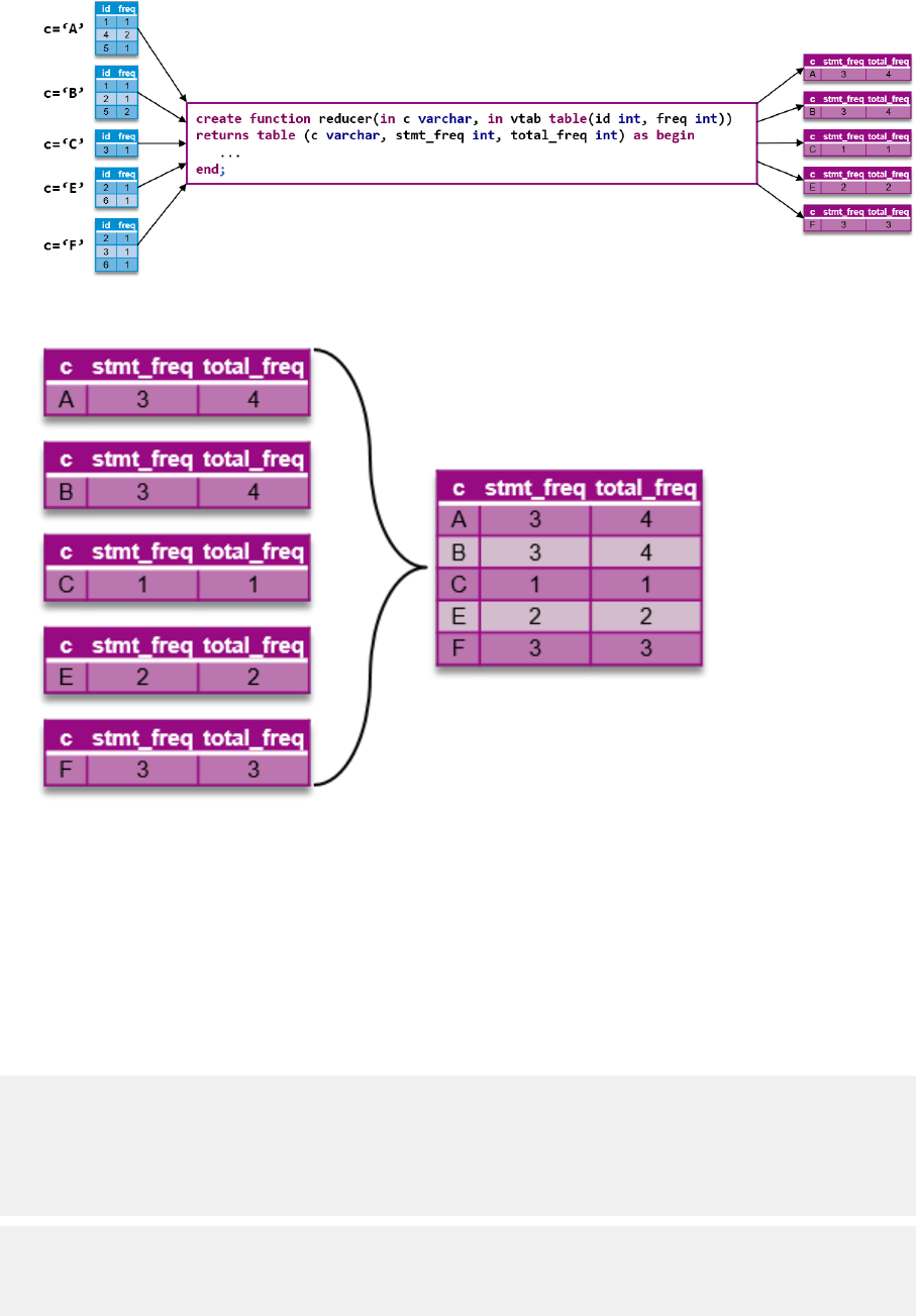
6. When all groups are processed, the output tables of the reducer are aggregated into a single big table (or
multiple tables, if the reducer is a procedure).
Retrieving Multiple Outputs from MAP_REDUCE
If you use a read-only procedure as a reducer, you can fetch multiple table outputs from a MAP_REDUCE
operator. To bind the output of MAP_REDUCE operators, you can simply apply the table variable as the
parameter of the reducer specication. For example, if you want to change the reducer in the example above to
a read-only procedure, apply the following code.
create procedure reducer_procedure(in c varchar, in values table(id int, freq
int), out otab table (c varchar, stmt_freq int, total_freq int))
reads sql data as begin
otab = select :c as c, count(distinct(id)) as stmt_freq, sum(freq) as
total_freq from :values;
end;
do begin
declare result table(c varchar, stmt_freq int, total_freq int);
MAP_REDUCE(tab, mapper(tab.id, tab.sentence) group by c as X,
reducer_procedure(X.c, X, result));
160
P U B L I C
SAP HANA Performance Guide for Developers
SQLScript Performance Guidelines

select * from :result order by c;
end;
Passing Extra Arguments as a Parameter to a Mapper or a Reducer
It is possible to pass extra arguments as parameters of a mapper or a reducer.
Sample Code
create function mapper(in id int, in sentence varchar(5000), in
some_extra_arg1 int, in some_extra_arg2 table(...), ...)
returns table (id int, c varchar, freq int) as begin
...
end;
create function reducer(in c varchar, in values table(id int, freq int), in
some_extra_arg1 int, in some_extra_arg2 table(...), ...)
returns table (c varchar, stmt_freq int, total_freq int) as begin
...
end;
do begin
declare result table(c varchar, stmt_freq int, total_freq int);
declare extra_arg1, extra_arg2 int;
declare extra_arg3, extra_arg4 table(...);
... more extra args ...
result = MAP_REDUCE(tab, mapper(tab.id,
tab.sentence, :extra_arg1, :extra_arg3, ...) group by c as X,
reducer(X.c, X, :extra_arg2, :extra_arg4,
1+1, ...));
select * from :result order by c;
end;
Note
There is no restriction about the order of input table parameters, input column parameters, extra
parameters and so on. It is also possible to use default parameter values in mapper/reducer TUDFs or
procedures.
Restrictions
The following restrictions apply:
● Only Mapper and Reducer are supported (no other Hadoop functionalities like group comparator, key
comparator and so on).
● The alias ID in the mapper output and the ID in the Reducer TUDF (or procedure) parameter must be the
same.
● The Mapper must be a TUDF, not a procedure.
● The Reducer procedure should be a read-only procedure and cannot have scalar output parameters.
SAP HANA Performance Guide for Developers
SQLScript Performance Guidelines
P U B L I C 161
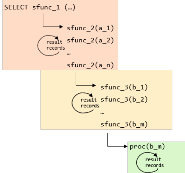
● The order of the rows in the output tables is not deterministic.
Related Information
Map Merge Operator [page 154]
6.7 Replacing Row-Based Calculations with Set-Based
Calculations
Row-based calculations are costly, particularly when they involve multiple nested loops. It is highly
recommended to rewrite them as set-based calculations. In the example below, which is a simplied illustration
of a real-life example, performance was improved by a factor of 85 through rewriting.
1. Compare the high-level overviews of the row-based calculation and set-based calculation.
The original scenario uses cursors with scalar functions. The scalar functions are called for each row. This
is repeated within the nested loops (n iterations each time):
162
P U B L I C
SAP HANA Performance Guide for Developers
SQLScript Performance Guidelines
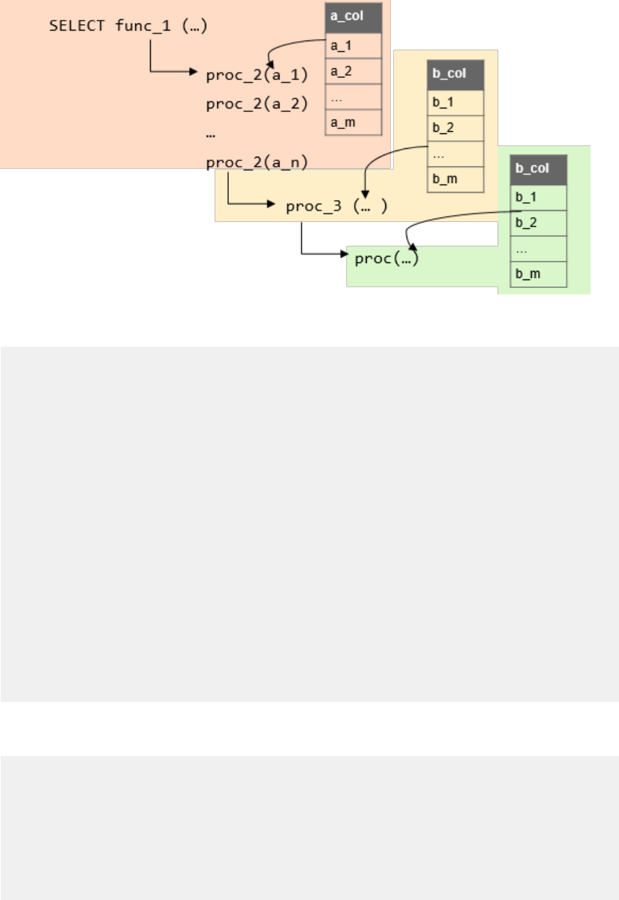
Below, the scalar functions are rewritten as procedures. All values are contained in tables:
2. Operate on a set of values.
The original scenario uses the cursor C1 to do a row-by-row calculation for each B value:
CREATE FUNCTION sfunc2(...)
RETURNS v_result NVARCHAR(2)
AS
CURSOR c1 FOR
SELECT *
FROM (SELECT SFUNC_3( :A, ip.B , :im_cti, :im_ci, :im_rd, :im_sp) AS C
,ip.*
,view1.esi
,view1.esti
,view1.au
FROM ( SELECT ...
FROM table_pes es
,table_es stat WHERE es.si = :A
AND es.ensi = stat.ensi
) view1
RIGHT OUTER JOIN (...) ip ON view1.B = ip.B);
BEGIN
FOR rec AS c1 DO
IF (rec.C = 1 OR rec.C = 3 ) THEN
ex_result := rec.C;
RETURN;
END IF;
END FOR;
ex_result := NULL;
END;
Below, the cursor C1 is replaced by a table assignment TAB_B. The function SFUNC_3 is rewritten as a
table function PROC_3 that takes TAB_B as an input. All statuses are calculated at once:
CREATE PROCEDURE proc2(..., OUT v_result NVARCHAR(2) )
READS SQL DATA AS
BEGIN
TAB_B = SELECT ip.B , ,ip.*,view1.esi,view1.esti,view1.au
FROM ( SELECT ...
FROM table_pes es
,table_es stat WHERE es.si = :A
AND es.ensi = stat.ensi
) view1
RIGHT OUTER JOIN (...) ip ON view1.B = ip.B;
SAP HANA Performance Guide for Developers
SQLScript Performance Guidelines
P U B L I C 163

CALL PROC_3(:A,:TAB_B,:im_cti,:im_ci,:im_rd,:im_sp, TAB_C);
TAB_RES = SELECT max(C) FROM :TAB_C where C in (1,3);
IF (NOT IS_EMPTY(:TAB_RES)) THEN
ex_result = :TAB_C.C[1];
RETURN;
END IF;
ex_result := NULL;
END
3. Filter a set of values.
The original scenario uses the cursor enr1 to iterate over a set of values and lter by B:
CURSOR enrl FOR
SELECT schd_id,...
FROM ...
WHERE enrl.schd_id = :p_schd_id;
FOR enrlrec AS enrl DO
...
SELECT COUNT(*) AS t_count INTO var_sc
FROM table_shd b,
table_pes c ,
table_schdr d,
table_cm e,
table_schdr f,
table_es g
WHERE
e.cti = :im_cti
AND e.ci = :im_ci
AND e.rev_dte = :im_rd
AND f.shi = :B
AND b.cti = :im_cti
AND b.act_ci = :im_ci
AND b.rev_dte = :im_rd
AND c.si = :A
AND d.shi = b.shi
AND ABS(DAYS_BETWEEN(d.ed ,f.sd))< COALESCE(e.sdtd,0)
AND c.esi = g.esi
AND g.esti != 'C';
...
END FOR;
Below the B lter is replaced by a GROUP BY clause. A left outer join is used to lter the result:
...
t1 = SELECT f.B AS shi, count(f.B) AS t_count
FROM table_shd b,
table_pes c ,
table_schdr d,
table_cm e,
table_schdr f,
table_es g
WHERE
e.cti = :im_cti
AND e.ci = :im_ci
AND e.rev_dte = :im_rev_dte
AND c.A = A
AND b.cti = :im_cti
AND b.act_ci = :im_ci
AND b.rev_dte = :im_rev_dte
AND d.B = b.B
AND ABS(DAYS_BETWEEN(d.ed ,f.sd))< COALESCE(e.sdtd,0)
AND c.esi = g.esi
AND g.esti != 'C'
GROUP BY f.B;
t2 = SELECT a.B, b.t_count
FROM :TAB_B as a
164
P U B L I C
SAP HANA Performance Guide for Developers
SQLScript Performance Guidelines

LEFT OUTER JOIN :t1 b
ON a.B = b.shi ORDER BY a.B;
...
6.8 Avoiding Busy Waiting
Avoid busy waiting situations by using the SLEEP_SECONDS and WAKEUP_CONNECTION procedures
contained in the SQLSCRIPT_SYNC built-in library.
In some scenarios you might need to let certain processes wait for a while (for example, when executing
repetitive tasks). Implementing such waiting manually might lead to busy waiting and to the CPU performing
unnecessary work during the waiting time.
Compare the following examples:
Problematic: Busy Wait
CREATE PROCEDURE WAIT( IN interval INT)
AS
BEGIN
DECLARE start_time TIMESTAMP = CURRENT_TIMESTAMP;
WHILE SECONDS_BETWEEN(start_time, CURRENT_TIMESTAMP) < :interval
DO
END WHILE;
END;
CREATE PROCEDURE MONITOR AS
BEGIN
WHILE 1 = 1 DO
IF RECORD_COUNT(OBSERVED_TABLE) > 100000 THEN
INSERT INTO LOG_TABLE VALUES (CURRENT_TIMESTAMP,
'Table size exceeds 100000 records');
END IF;
CALL WAIT (300);
END WHILE;
END
Recommended: Sleep Procedure
SAP HANA Performance Guide for Developers
SQLScript Performance Guidelines
P U B L I C 165

DO BEGIN
USING SQLSCRIPT_SYNC AS SYNC;
DECLARE i INTEGER;
lt_con = SELECT connection_id AS CON_ID
FROM M_SERVICE_THREADS
WHERE lock_wait_name like 'SQLSCRIPT_WAIT%';
FOR i in 1..record_count(:lt_con) DO
CALL SYNC:WAKEUP_CONNECTION(:lt_con.CON_ID[:i]);
END FOR;
END;
CREATE PROCEDURE MONITOR AS
BEGIN
USING SYS.SQLSCRIPT_SYNC AS SYNC;
WHILE 1 = 1 DO
IF RECORD_COUNT(OBSERVED_TABLE) > 100000 THEN
INSERT INTO LOG_TABLE VALUES (CURRENT_TIMESTAMP,
'Table size exceeds 100000 records');
END IF;
CALL SYNC:SLEEP_SECONDS(300);
END WHILE;
END
● In the rst example, a WAIT procedure denes a period during which a process simply waits. In the
MONITOR procedure, WAIT is used to make the process wait for 300 seconds before it resumes. This
means that the thread is active all the time.
● In the second example, the SLEEP_SECONDS and WAKEUP_CONNECTION procedures are used as
follows:
○ First, the SQLSCRIPT_SYNC library is referenced with USING SQLSCRIPT_SYNC.
○ The WAKEUP_CONNECTION procedure is used to resume all sleeping processes.
A sleeping process is listed in the monitoring view M_SERVICE_THREADS. Its LOCK_WAIT_NAME
starts with 'SQLScript/SQLScript_Sync/Sleep/'.
○ The SLEEP_SECONDS procedure is used to pause the execution of the current process for the
specied waiting time in seconds.
6.9 Best Practices for Using SQLScript
The following best practices help to enhance the performance of SQLScript procedures.
Related Information
Reduce the Complexity of SQL Statements [page 167]
Identify Common Sub-Expressions [page 167]
Multi-Level Aggregation [page 167]
Reduce Dependencies [page 168]
Avoid Using Cursors [page 168]
Avoid Using Dynamic SQL [page 170]
166
P U B L I C
SAP HANA Performance Guide for Developers
SQLScript Performance Guidelines

6.9.1 Reduce the Complexity of SQL Statements
Variables in SQLScript enable you to arbitrarily break up a complex SQL statement into many simpler ones.
This makes a SQLScript procedure easier to comprehend.
To illustrate this point, consider the following query:
books_per_publisher = SELECT publisher, COUNT (*) AS cnt
FROM :books GROUP BY publisher;
largest_publishers = SELECT * FROM :books_per_publisher
WHERE cnt >= (SELECT MAX (cnt)
FROM :books_per_publisher);
Writing this query as a single SQL statement requires either the denition of a temporary view (using WITH), or
the multiple repetition of a sub-query. The two statements above break the complex query into two simpler
SQL statements that are linked by table variables. This query is much easier to understand because the names
of the table variables convey the meaning of the query and they also break the complex query into smaller
logical pieces.
The SQLScript compiler will combine these statements into a single query or identify the common sub-
expression using the table variables as hints. The resulting application program is easier to understand without
sacricing performance.
6.9.2 Identify Common Sub-Expressions
The query examined in the previous topic contained common sub-expressions. Such common sub-expressions
might introduce expensive repeated computation that should be avoided.
It is very complicated for query optimizers to detect common sub-expressions in SQL queries. If you break up a
complex query into logical subqueries it can help the optimizer to identify common sub-expressions and to
derive more ecient execution plans. If in doubt, you should employ the EXPLAIN plan facility for SQL
statements to investigate how the SAP HANA database handles a particular statement.
6.9.3 Multi-Level Aggregation
Computing multi-level aggregation can be achieved by using grouping sets. The advantage of this approach is
that multiple levels of grouping can be computed in a single SQL statement.
For example:
SELECT publisher, name, year, SUM(price)
FROM :it_publishers, :it_books
WHERE publisher=pub_id AND crcy=:currency
GROUP BY GROUPING SETS ((publisher, name, year), (year))
To retrieve the dierent levels of aggregation, the client must typically examine the result repeatedly, for
example, by ltering by NULL on the grouping attributes.
In the special case of multi-level aggregations, SQLScript can exploit results at a ner grouping for computing
coarser aggregations and return the dierent granularities of groups in distinct table variables. This could save
SAP HANA Performance Guide for Developers
SQLScript Performance Guidelines
P U B L I C 167

the client the eort of re-examining the query result. Consider the above multi-level aggregation expressed in
SQLScript:
books_ppy = SELECT publisher, name, year, SUM(price)
FROM :it_publishers, :it_books
WHERE publisher = pub_id AND crcy = :currency
GROUP BY publisher, name, year;
books_py = SELECT year, SUM(price)
FROM :books_ppy
GROUP BY year;
6.9.4 Reduce Dependencies
One of the most important methods for speeding up processing in the SAP HANA database is through
massively parallelized query execution.
Parallelization is exploited at multiple levels of granularity. For example, the requests of dierent users can be
processed in parallel, and single relational operators within a query can also be executed on multiple cores in
parallel. It is also possible to execute dierent statements of a single SQLScript procedure in parallel if these
statements are independent of each other. Remember that SQLScript is translated into a dataow graph, and
independent paths in this graph can be executed in parallel.
As an SQLScript developer, you can support the database engine in its attempt to parallelize execution by
avoiding unnecessary dependencies between separate SQL statements, and by using declarative constructs if
possible. The former means avoiding variable references, and the latter means avoiding imperative features,
such as cursors.
6.9.5 Avoid Using Cursors
While the use of cursors is sometime required, they also imply row-by-row processing. Consequently,
opportunities for optimizations by the SQL engine are missed. You should therefore consider replacing cursors
with loops in SQL statements.
Read-Only Access
For read-only access to a cursor, consider using simple selects or joins:
CREATE PROCEDURE foreach_proc LANGUAGE SQLSCRIPT AS
Reads SQL DATA
BEGIN
DECLARE val decimal(34,10) = 0;
DECLARE CURSOR c_cursor1 FOR
SELECT isbn, title, price FROM books;
FOR r1 AS c_cursor1 DO
val = :val + r1.price;
END FOR;
END;
168
P U B L I C
SAP HANA Performance Guide for Developers
SQLScript Performance Guidelines

This sum can also be computed by the SQL engine:
SELECT sum(price) into val FROM books;
Computing this aggregate in the SQL engine may result in parallel execution on multiple CPUs inside the SQL
executor.
Updates and Deletes
For updates and deletes, consider using the following:
CREATE PROCEDURE foreach_proc LANGUAGE SQLSCRIPT AS
BEGIN
DECLARE val INT = 0;
DECLARE CURSOR c_cursor1 FOR
SELECT isbn, title, price FROM books;
FOR r1 AS c_cursor1 DO
IF r1.price > 50 THEN
DELETE FROM Books WHERE isbn = r1.isbn;
END IF;
END FOR;
END;
This delete can also be computed by the SQL engine:
DELETE FROM Books
WHERE isbn IN (SELECT isbn FROM books WHERE price > 50);
Computing this in the SQL engine reduces the calls through the runtime stack of the SAP HANA database. It
also potentially benets from internal optimizations like buering and parallel execution.
Insertion into Tables
CREATE PROCEDURE foreach_proc LANGUAGE SQLSCRIPT AS
BEGIN
DECLARE val INT = 0;
DECLARE CURSOR c_cursor1 FOR SELECT isbn, title, price FROM books;
FOR r1 AS c_cursor1 DO
IF r1.price > 50
THEN
INSERT INTO ExpensiveBooks VALUES(..., r1.title, ...);
END IF;
END FOR;
END;
This insertion can also be computed by the SQL engine:
SELECT ..., title, ... FROM Books WHERE price > 50
INTO ExpensiveBooks;
Like updates and deletes, computing this statement in the SQL engine reduces the calls through the runtime
stack of the SAP HANA database. It also potentially benets from internal optimizations like buering and
parallel execution.
SAP HANA Performance Guide for Developers
SQLScript Performance Guidelines
P U B L I C 169

6.9.6 Avoid Using Dynamic SQL
Dynamic SQL is a powerful way to express application logic. It allows SQL statements to be constructed at the
execution time of a procedure. However, executing dynamic SQL is slow because compile-time checks and
query optimization must be performed each time the procedure is called. When there is an alternative to
dynamic SQL using variables, this should be used instead.
Another related problem is security because constructing SQL statements without proper checks of the
variables used can create a security vulnerability, like an SQL injection, for example. Using variables in SQL
statements prevents these problems because type checks are performed at compile time and parameters
cannot inject arbitrary SQL code.
The table below summarizes potential use cases for dynamic SQL:
Table 9: Dynamic SQL Use Cases
Feature
Proposed Solution
Projected attributes Dynamic SQL
Projected literals SQL + variables
FROM clause
SQL + variables; result structure must remain unchanged
WHERE clause – attribute names and Boolean operators APPLY_FILTER
170 P U B L I C
SAP HANA Performance Guide for Developers
SQLScript Performance Guidelines
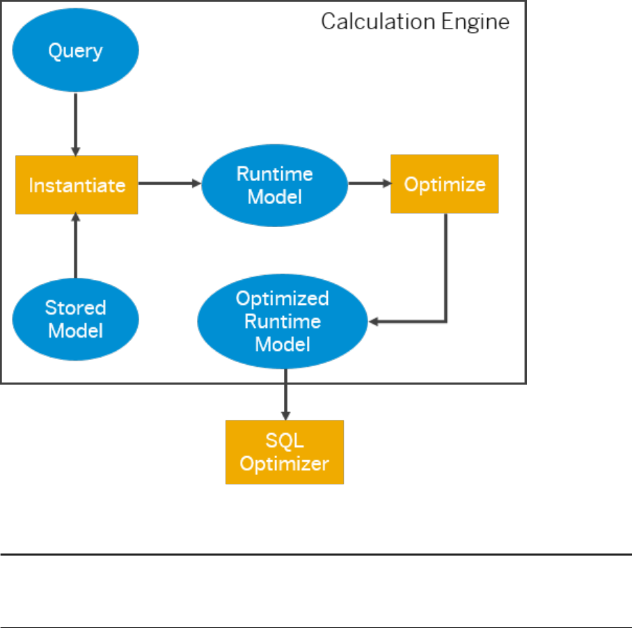
7 Optimization Features in Calculation
Views
The calculation engine pre-optimizes queries before they are worked on by the SQL optimizer.
As shown in the overview below, a calculation view is instantiated at runtime when a query is executed. During
the instantiation process, the calculation engine simplies the calculation view into a model that fullls the
requirements of the query. This results in a reduced model that can be further optimized by the calculation
engine. After this, the SQL optimizer applies further optimizations and determines the query execution plan:
Some of the main optimization features include the following:
Feature
Description
Join cardinality The specied join cardinality allows the optimizer to decide whether a
join needs to be executed. In models in which many joins are dened, join
pruning can lead to a signicant performance boost and reduction in
temporary memory consumption.
SAP HANA Performance Guide for Developers
Optimization Features in Calculation Views
P U B L I C 171

Feature Description
Optimized join columns By explicitly allowing join columns to be optimized, you can potentially re
duce the number of records that need to be processed at later stages of
query processing, resulting in better performance and reduced resource
consumption.
Dynamic joins
Dynamic joins help improve the join execution process by reducing the
number of records processed by the join view node at runtime.
Union node pruning This allows the data sources of union nodes to be pruned, which helps re
duce resource consumption and benets performance.
Column pruning Column pruning is an intrinsic feature of calculation views. It automati
cally removes any columns that are not needed for the nal results during
the early stages of processing.
Note
In general, we recommend that you set a join cardinality and consider setting the Optimized Join Columns
ag.
Tip
Union node pruning has proved to be a helpful modeling pattern in many scenarios.
7.1 Calculation View Instantiation
Calculation views are processed by the calculation engine, during which it applies a variety of optimizations.
These can sometimes result in nonrelational behavior, that is, behavior that is not typical in SQL, and this in
turn can have an impact on performance. One of the reasons for non-relational behavior is the instantiation
process.
The instantiation process transforms a stored calculation model into an executed calculation model based on a
query that is run on top of a calculation view. The calculation view is technically a column view that references
one specic node of the stored calculation model. Therefore, during the instantiation process, the query and
the stored calculation model are combined to build the executed calculation model.
The main dierence between a relational view, or SQL with subselects, and a calculation model is that the
projection list in a relational view is stable even when another SQL statement is stacked on top of it. In a
calculation model, on the other hand, the projection list of each calculation node in the calculation model
depends on the columns requested by the query or the parent calculation node. The requested columns are
the superset of all columns that are used in the query, for example, the columns in the projection list, the
columns in the WHERE and HAVING clauses, the columns used for sorting, and the columns in the ON clause
for joins, and so on.
The following examples illustrate the dierence between the stored model, that is, the calculation view, and the
optimized model that results when the calculation view is matched to the query.
172
P U B L I C
SAP HANA Performance Guide for Developers
Optimization Features in Calculation Views
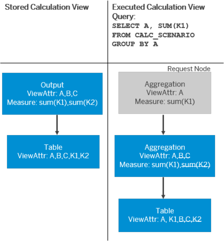
Example 1: Aggregration over a table
In this example, you can see that the table request contains only the attribute A and column K1 in its projection
list:
SAP HANA Performance Guide for Developers
Optimization Features in Calculation Views
P U B L I C 173
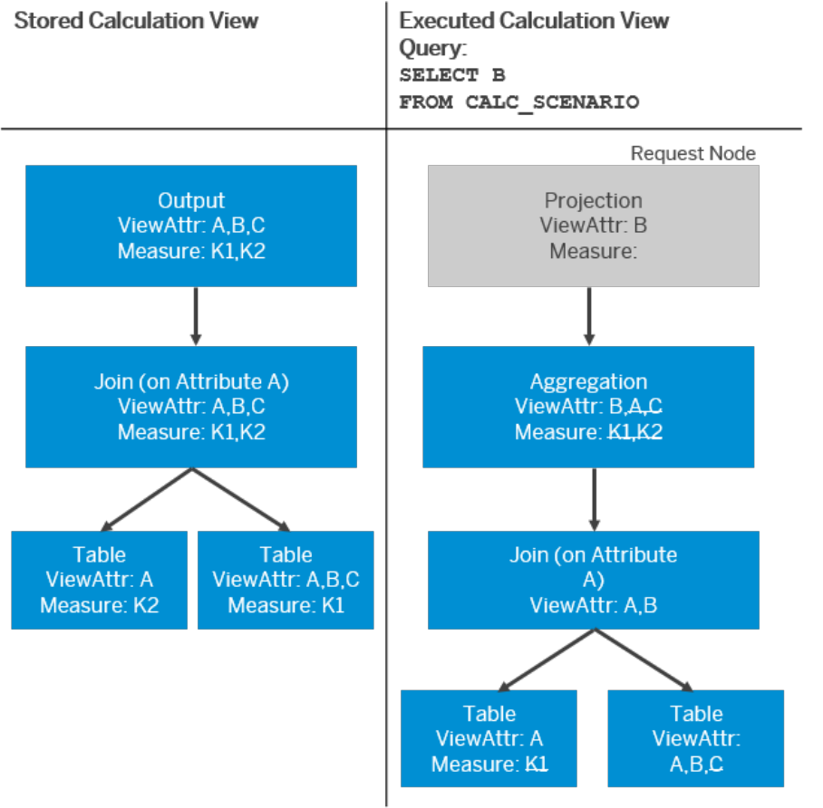
Example 2: Join over two tables
This example shows that the attribute A is added to the projection list at the join node and the underlying
nodes because it is required for the join:
Example 3: Dierent semantics
The semantics can change, depending on which attributes and columns are requested. In this example, a
calculated attribute is dened on the aggregation node in the middle. You can see that in the aggregation over
the table, the attribute A is added to the projection list. The reason for this is the presence of the calculated
174
P U B L I C
SAP HANA Performance Guide for Developers
Optimization Features in Calculation Views
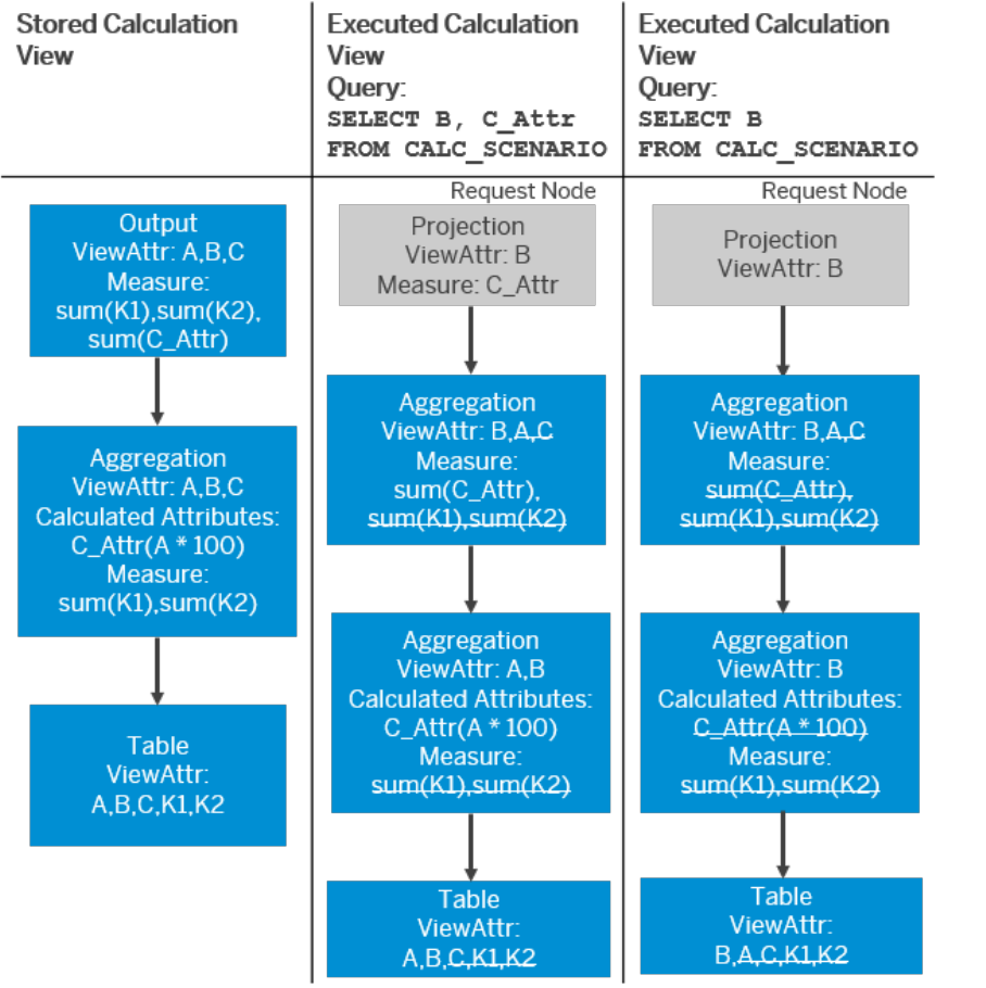
attribute C_Attr. When the calculated attribute is not queried, the attribute A is not added to the projection list
of the aggregation:
SAP HANA Performance Guide for Developers
Optimization Features in Calculation Views
P U B L I C 175
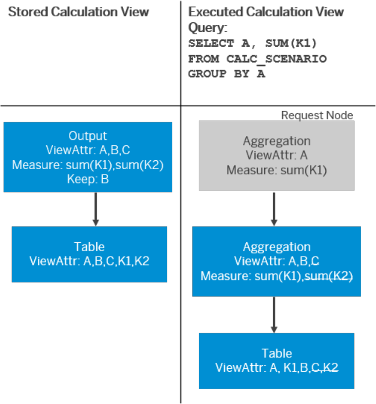
Example 4: Enforcing attributes using the keep ag
To force an attribute to be requested irrespective of the projection list of the parent node, you can set the keep
ag for this attribute. The eect of the keep ag on the executed model in example 1 is shown below. Now the
attribute B is requested on the lower nodes, despite not being requested by the query:
7.2 Setting Join Cardinality
A specied join cardinality allows the optimizer to decide based on the elds requested in the query whether a
join needs to be executed. In models in which many joins are dened, join pruning can lead to signicant
performance boosts and reductions in temporary memory consumption.
Imagine a dened star join involving 100 or more tables through further join chains. If no dimensional values
are requested and the cardinality setting is n..1 or 1..1, all joins can be omitted. As a result, the query can be
reduced to one single table access to the central table, instead of involving all the potential join cascades.
176
P U B L I C
SAP HANA Performance Guide for Developers
Optimization Features in Calculation Views
Note, however, that while join pruning allows performance to be improved and resource consumption reduced,
there is also a risk that it will return surprising results if the cardinality setting does not reect the actual
cardinality of the data. Also, should the data cardinality change at any stage, for example, due to data
remodeling or data loading, the cardinality setting will need to be adjusted. Ideally, your data loading process
should ensure that the specied cardinality is upheld.
7.2.1 Join Cardinality
A cardinality setting can be applied to joins in calculation views. It species for each entry in one table how
many matching entries there are in the other table of the join.
Join cardinality is denoted using two numbers. The left number describes the number of matching entries for
the entries in the right table, while the right number describes the number of matching entries for the entries in
the left table. For example, there is a join on the EMPLOYEE eld between table 1 (left table) and table 2 (right
table):
● A join cardinality of 1..n species that table 2 has at most one matching entry in table 1. Conversely, each
entry in table 1 can have zero to n matching entries in table 2. The symbol n denotes an arbitrary positive
number. For example, the entry Alice in table 1 might have zero, one, or an arbitrary number of matches in
table 2.
● A join cardinality of 1..1 indicates that each entry in table 1, for example, the entry Alice in table 1, has zero
or one matching entry in table 2. In the same way, the entry Alice in table 2 also has at most one match in
table 1.
Join Pruning Prerequisites
The cardinality setting is used by the optimizer to decide, based on the elds requested in the query, whether a
join needs to be executed or whether it can be omitted without comprising the correctness of the data. A join
can be omitted if executing the join does not add or remove any records, and provided that no elds are
requested from the table that is to be omitted.
While inner joins can add records (multiple matching entries in the other table) and remove records (no
matching entry, remember that ..1 includes zero), outer joins can only add records. Therefore, by using join
cardinality to ensure that the table to be pruned has at most one matching item, you allow join pruning to occur
for outer joins. Text joins behave like left-outer joins in this respect. In the case of referential joins, pruning can
only occur if the referential integrity is set for the table that is not to be pruned. Note that the referential
integrity can be placed on the left table, the right table, or on both tables.
There is one exception to the rule that requires that the table to be pruned has a setting of ..1. This applies
when the query only requests measures with the count distinct aggregation mode. In this case, any repeated
values that could potentially exist in the tables to be pruned are made unique again by the count distinct
calculation. Consequently, join execution does not change the results of the count distinct measure even if
there is an n..m cardinality.
All the following prerequisites therefore need to be met for join pruning to occur:
● No elds are requested from the table to be pruned.
SAP HANA Performance Guide for Developers
Optimization Features in Calculation Views
P U B L I C 177

● The join type is either an outer join, a referential join with integrity on the table that is not to be pruned, or a
text join where the table to be pruned contains the language column.
● The join cardinality is either ..1 for the table to be pruned, or the query only requests measures with count
distinct aggregation or does not request any measures at all.
Join Cardinality Proposals
If tables are directly involved in the join, cardinality proposals can be obtained from the modeling tool. These
values are based on the data cardinality at the time of the proposal. These proposals are not available if the join
includes further nodes (for example, the table is added through a projection node).
Irrespective of whether the cardinality setting is achieved through a proposal or manual setting, the optimizer
relies on these values when making decisions about join pruning. There are no runtime checks. If the setting
gives a lower cardinality than the actual cardinality of the data (for example, it is set to n..1, but in the data it is
n..m), omitting the join might lead to changes in the measure values, compared to when the join is executed.
7.2.2 Examples
The following examples demonstrate how the join cardinality setting can inuence the outcome of queries.
All examples are based on two tables and a join between these two tables. In some examples, additional
projection or aggregation nodes are added. Otherwise, the examples are intentionally simple to illustrate the
mechanisms at work. Obviously, performance gains cannot be observed in these simple models, even though
they exist.
Related Information
Example Tables [page 178]
Get Join Cardinality Proposals [page 179]
Impact of Join Cardinality on Pruning Decisions [page 181]
Impact of Incorrect Join Cardinality Settings [page 189]
7.2.2.1 Example Tables
These two tables are used in all the examples.
SalesOrders
SALESORDER EMPLOYEE AMOUNT
001 Donald 20
178 P U B L I C
SAP HANA Performance Guide for Developers
Optimization Features in Calculation Views

SalesOrders
SALESORDER EMPLOYEE AMOUNT
002 Alice 22
003 Hans 40
004 Horst 33
Employees
MANAGER EMPLOYEE
null Alice
Alice Donald
Alice Dagobert
Alice Hans
Hans Heinz
Hans Jane
? Horst
As you can see, there is a 1..1 relationship between the EMPLOYEE eld in the SalesOrders table and the
EMPLOYEE eld in the Employees table. In contrast, there is a 1..n relationship between the EMPLOYEE eld in
the SalesOrders table and the MANAGER eld in the Employees table.
7.2.2.2 Get Join Cardinality Proposals
In this example, the modeling tool is used to get a proposal for the join cardinality. The proposal is derived from
the data cardinality applicable for the join elds between the tables at the time of the proposal. To get a
cardinality proposal, the join must be based directly on tables.
Procedure
1. Create a calculation view.
Create a calculation view that only includes a join between the SalesOrders and Employees tables. Join the
two tables with a left outer join on the EMPLOYEE eld, where the SalesOrders table is the left table:
SAP HANA Performance Guide for Developers
Optimization Features in Calculation Views
P U B L I C 179
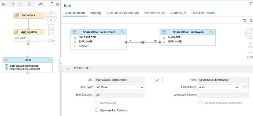
Note that the Cardinality eld above has a Propose Cardinality button for requesting proposals.
As described earlier, the SalesOrders table only has distinct values in the EMPLOYEE column. Similarly, the
EMPLOYEE column in the Employees table also has no repeated values. Therefore, if you wanted to set the
cardinality for a join on the EMPLOYEE elds, you would set it to 1..1. Since only tables are involved in this
join, you can now get the cardinality proposals.
2. Get a join cardinality proposal:
a. To get a join cardinality proposal, click the Propose Cardinality button.
Based on the cardinality of the EMPLOYEE eld in both tables, 1..1 is proposed.
b. For the purposes of the example, remove the join and create a new left-outer join, this time between
the EMPLOYEE eld in the left table and the manager eld in the right table.
c. Get a new join cardinality proposal.
Since there are multiple duplicates in the manager column (for example, Alice), the tool proposes
1..n.
The modeler therefore proposes a cardinality for the join eld based on the current data cardinality,
provided you have only included tables in your join.
3. To see that join cardinality proposals are not available if the join includes other nodes, create another
calculation view.
a. This time do not add the Employees table directly to the join node, but place it in a projection, as shown
below:
180
P U B L I C
SAP HANA Performance Guide for Developers
Optimization Features in Calculation Views
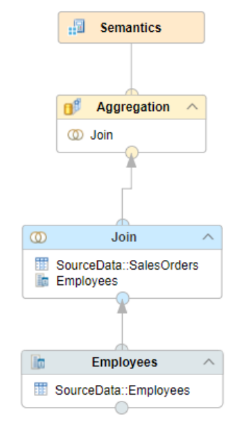
b. Request a join cardinality proposal.
The Propose Cardinality button is now grayed out. This is because a proposal is only available when
tables are joined directly. In this example, one table is joined indirectly through a projection.
This example has therefore demonstrated that join cardinality proposals are only supported when tables
are directly involved in the join and are not passed up through other nodes.
7.2.2.3 Impact of Join Cardinality on Pruning Decisions
The following examples demonstrate how setting the join cardinality in calculation view joins can lead to join
pruning and thus better performance.
Related Information
Example 1: All pruning conditions are satised [page 182]
Example 2: Additional eld is requested from the right table [page 183]
Example 3: Dierent cardinality settings [page 184]
Example 4: Requested measures [page 186]
SAP HANA Performance Guide for Developers
Optimization Features in Calculation Views
P U B L I C 181
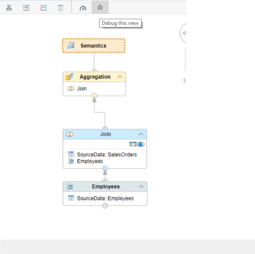
7.2.2.3.1 Example 1: All pruning conditions are satised
Join pruning can occur when all pruning conditions are satised.
Procedure
1. Manually set the cardinality of the calculation view developed earlier in Get Join Cardinality Proposals to
1..1 and add all elds so you can build the calculation view.
2. Make sure that the EMPLOYEE_1 eld comes from the left table. If this is not the case, for example, because
you built the model in a slightly dierent way, change the column mapping in the join node so that
EMPLOYEE_1 refers only to the left table.
3. After the calculation view has been built, start debugging by selecting the Semantics node and then
choosing the Debug button:
4. Replace the default debug query with a query that only requests elds from the left table and run the query
(you probably need to change the calculation view name):
SELECT
"SALESORDER",
182
P U B L I C
SAP HANA Performance Guide for Developers
Optimization Features in Calculation Views
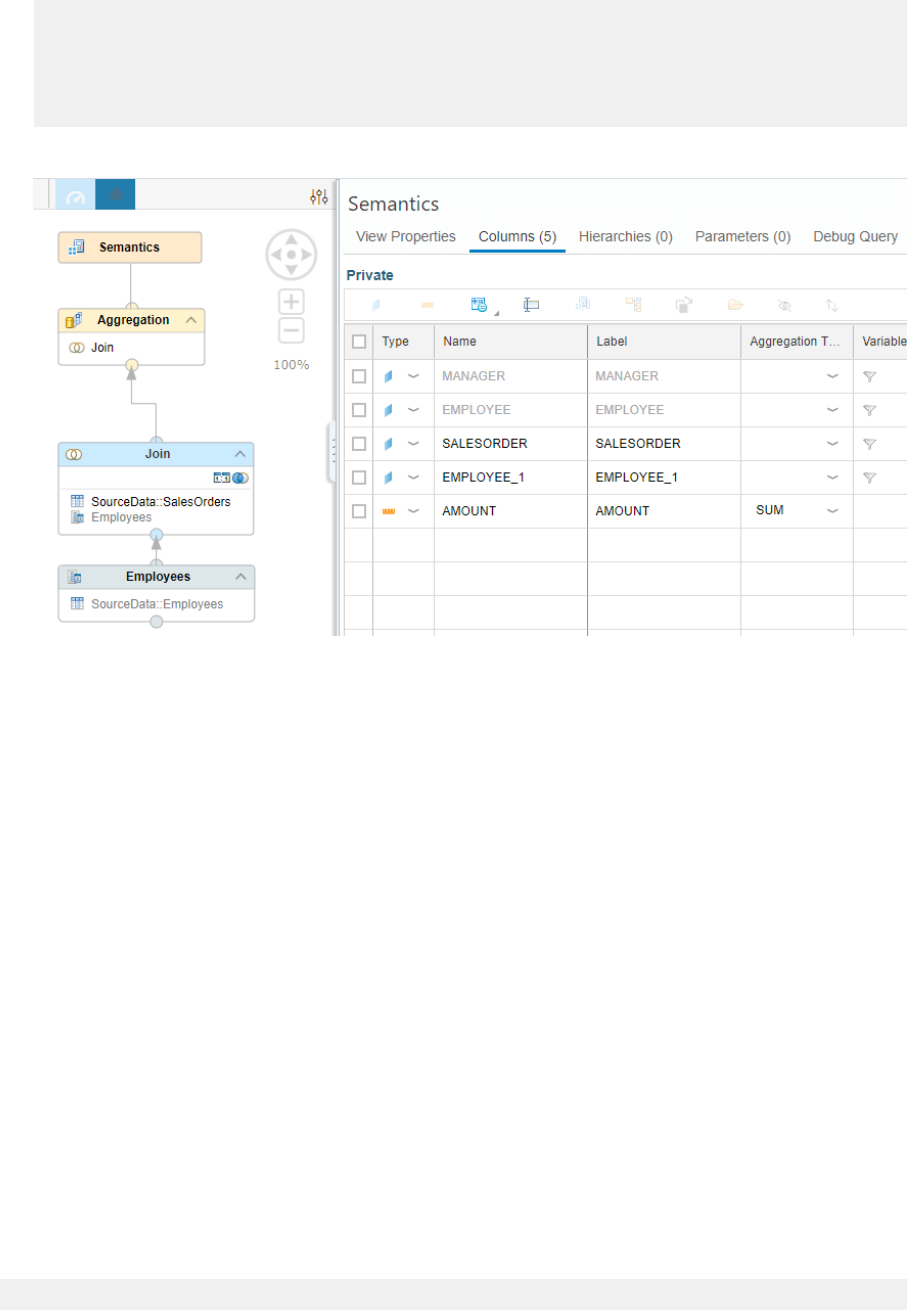
"EMPLOYEE_1",
SUM("AMOUNT") AS "AMOUNT"
FROM
"JOINCARDINALITY_1"."joinCardinalityExample.db.CVs::joinCardinalityNoEstimate"
GROUP BY
"SALESORDER","EMPLOYEE_1"
The executed debug query shows the pruned nodes and elds in gray:
Based on the grayed-out objects, you can conclude that the employees table was pruned away.
Pruning could occur because all the following conditions were met:
○ No elds were requested from Employees (EMPLOYEE_1 comes from the left table).
○ Only left-outer joins were involved, which meant that records could not be removed by executing the
join.
○ The cardinality was set such that the number of records would not be expected to increase by
executing the join.
7.2.2.3.2 Example 2: Additional eld is requested from the
right table
If you include elds from the right table (for example, the MANAGER eld), join pruning cannot occur because
the join has to be executed to associate the records from both tables.
Procedure
To test this, run the following debug query that additionally requests the MANAGER eld from the right table:
SELECT
SAP HANA Performance Guide for Developers
Optimization Features in Calculation Views
P U B L I C 183
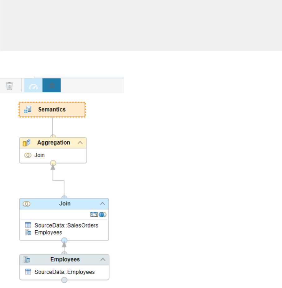
"SALESORDER",
"EMPLOYEE_1",
"MANAGER",
SUM("AMOUNT") AS "AMOUNT"
FROM
"JOINCARDINALITY_1"."joinCardinalityExample.db.CVs::joinCardinalityNoEstimate"
GROUP BY
"SALESORDER","EMPLOYEE_1","MANAGER"
As you can see, this debug query prevents pruning. The Employees table is not grayed out, conrming that it
was not pruned:
7.2.2.3.3 Example 3: Dierent cardinality settings
To see more demonstrations of the impact of the cardinality setting on join pruning, set the cardinality to the
following values sequentially before running the debug queries below:
1. n..1
2. 1..n
3. Leave it empty
Don’t forget to save and build the calculation view each time.
184
P U B L I C
SAP HANA Performance Guide for Developers
Optimization Features in Calculation Views
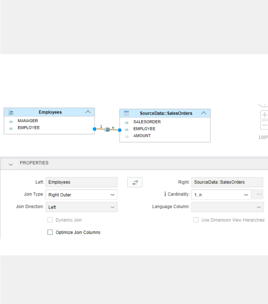
Procedure
1. Run the following debug query, which only accesses the left table:
SELECT
"SALESORDER",
"EMPLOYEE_1",
SUM("AMOUNT") AS "AMOUNT"
FROM
"JOINCARDINALITY_1"."joinCardinalityExample.db.CVs::joinCardinalityNoEstimate"
GROUP BY
"SALESORDER","EMPLOYEE_1"
You should see that pruning only occurs with a left-outer join and n..1 (or 1..1 from before). As
discussed above, inner joins prevent pruning.
2. In the same way for right-outer joins, only 1..1 and 1..n work. To check, swap the join sides by choosing
the Swap Table button.
3. Dene a right outer join with the cardinality 1..n:
4. Run the following debug query, for example:
SELECT
"EMPLOYEE_1",
SUM("AMOUNT") AS "AMOUNT"
FROM
"JOINCARDINALITY_1"."joinCardinalityExample.db.CVs::joinCardinalityRightOuter"
GROUP BY
"EMPLOYEE_1"
Join pruning should now occur.
SAP HANA Performance Guide for Developers
Optimization Features in Calculation Views
P U B L I C 185
7.2.2.3.4 Example 4: Requested measures
This example shows how the type of requested measure inuences the outcome. In the previous examples, join
pruning only worked when there was an outer-join setting and the table to be pruned had a cardinality of ..1.
Context
In this example, a cardinality of n..m also allows pruning to occur when the query only requests a count
distinct measure. The reason for this is that count distinct removes any potential duplicates and the outer join
ensures that no records are lost. In
SUM, since no records can be lost due to the outer join and potential
duplicate records do not inuence the outcome of the count distinct measure, executing the join does not
inuence the value of the measure. Therefore, the join can be omitted if no elds are requested from the table
to be pruned.
Procedure
1. For a working example, dene a calculated column of type count distinct on the EMPLOYEE_1 eld:
186
P U B L I C
SAP HANA Performance Guide for Developers
Optimization Features in Calculation Views
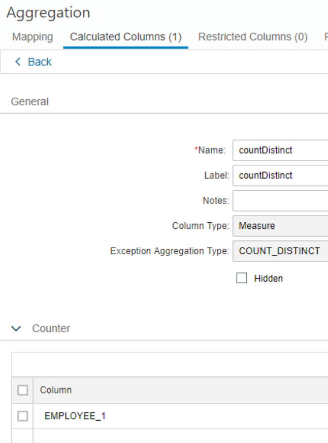
2. Set the cardinality to n..m:
SAP HANA Performance Guide for Developers
Optimization Features in Calculation Views
P U B L I C 187
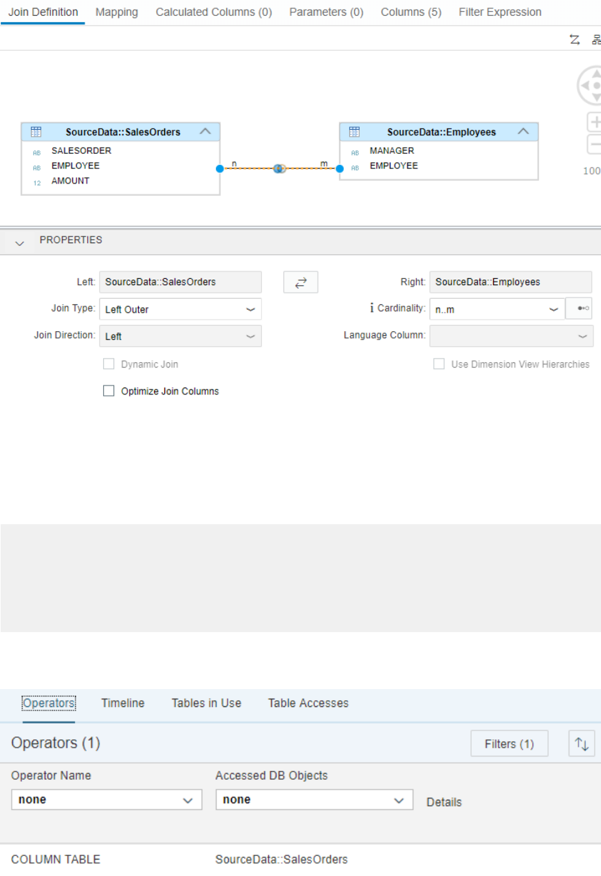
Debug queries that only request the count distinct measure and elds from the left table should now show
table pruning.
3. Instead of running the query in debug view, use the Database Explorer to check whether join pruning
occurs. Open the Database Explorer by clicking the Database Explorer button on the left.
4. Open an SQL console and enter the debug query, for example:
SELECT
"EMPLOYEE_1",
SUM("COUNTDISTINCT") AS "COUNTDISTINCT"
FROM
"JOINCARDINALITY_1"."joinCardinalityExample.db.CVs::JoinEstimateCardinalityCou
ntDistinct"
GROUP BY "EMPLOYEE_1"
5. From the Run dropdown menu, choose Analyze SQL.
On the Operators tab, you should see that only one table was used. For example:
188
P U B L I C
SAP HANA Performance Guide for Developers
Optimization Features in Calculation Views
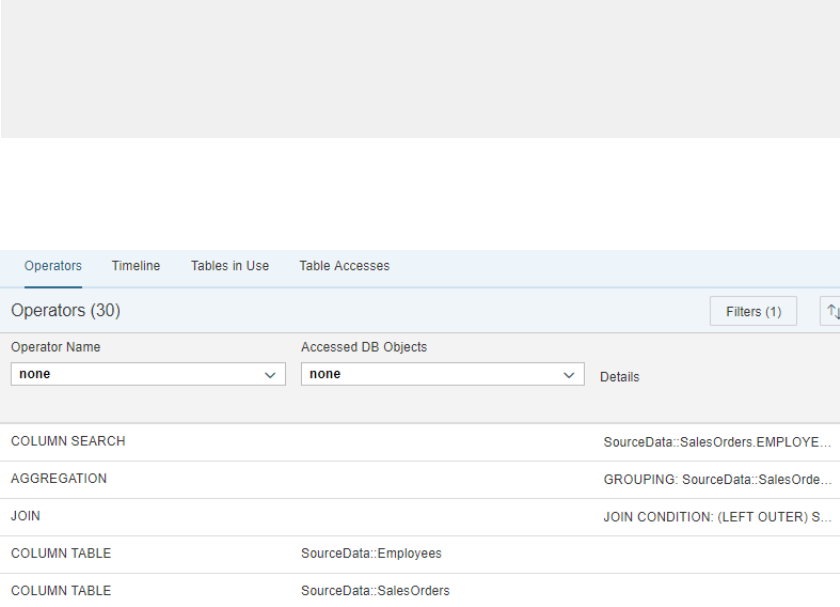
This demonstrates that join pruning also occurs with a cardinality setting of n..m when the only measure
used is of type count distinct.
6. Add an additional AMOUNT measure to the query to see that two tables are then involved:
a. Open an SQL console and enter the debug query, for example:
SELECT "EMPLOYEE_1", SUM("COUNTDISTINCT") AS "COUNTDISTINCT",
SUM("AMOUNT") AS "AMOUNT"
FROM
"JOINCARDINALITY_1"."joinCardinalityExample.db.CVs::JoinEstimateCardinality
CountDistinct"
GROUP BY "EMPLOYEE_1"
b. From the Run dropdown menu, choose Analyze SQL.
On the Operators tab, you should see that both tables are used and no join pruning occurs. For
example:
7.2.2.4 Impact of Incorrect Join Cardinality Settings
The three examples in this section illustrate how the resulting values of measures are aected depending on
whether join pruning occurs when an incorrect cardinality is dened. Each example shows dierent reasons for
the incorrect cardinalities: wrong from the outset, after remodeling, and after loading additional data.
Related Information
Example 1: Wrong from the Outset [page 190]
Example 2: Remodeling [page 192]
Example 3: Loading Additional Data [page 195]
SAP HANA Performance Guide for Developers
Optimization Features in Calculation Views
P U B L I C 189
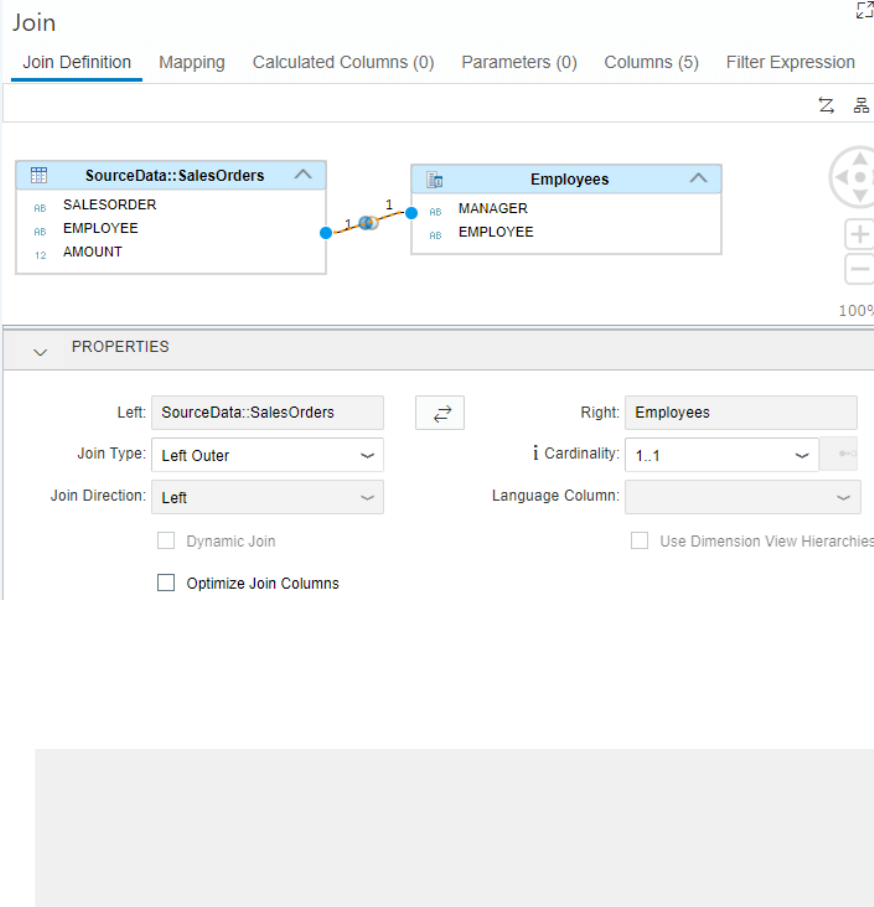
7.2.2.4.1 Example 1: Wrong from the Outset
This example shows how dierent results are obtained for the AMOUNT measure when the join is executed
because the cardinality is set incorrectly. In this case, the cardinality does not match the cardinality present in
the data.
Procedure
1. In the calculation view, set the cardinality of a left-outer join between the EMPLOYEE eld in the SalesOrders
table and the MANAGER eld in the Employees table to 1..1, as shown below:
The dened cardinality of 1..1 is not reected in the data, which leads to the problems shown in the next
steps.
2. Compare the results of the two queries below:
a. Query on elds from the left table only:
SELECT
"EMPLOYEE_1",
SUM("AMOUNT") AS "AMOUNT"
FROM
"JOINCARDINALITY_1"."joinCardinalityExample.db.CVs::joinCardinalityWrongFro
mOutset"
GROUP BY "EMPLOYEE_1"
190
P U B L I C
SAP HANA Performance Guide for Developers
Optimization Features in Calculation Views

b. Query on elds from both tables:
SELECT
"EMPLOYEE_1",
"MANAGER",
SUM("AMOUNT") AS "AMOUNT"
FROM
"JOINCARDINALITY_1"."joinCardinalityExample.db.CVs::joinCardinalityWrongFro
mOutset"
GROUP BY "EMPLOYEE_1","MANAGER"
Result: Query on Fields from the Left Table Only
Result: Query on Fields from Both Tables
EMPLOYEE_1 AMOUNT EMPLOYEE_1 MANAGER AMOUNT
Donald 20 Donald NULL 20
Alice 22 Alice Alice 66
Hans 40 Hans Hans 80
Horst 33 Horst NULL 33
As you can see, dierent values are obtained for the AMOUNT measure for both Alice and Hans:
○ In the rst query, join pruning can occur because all elds come from the left table and the cardinality
setting allows it. Because the join is not executed, the multiple entries matching Alice in the right table
are not found:
Left Table: SalesOrders
Right Table: Employees
SALESORDER EMPLOYEE AMOUNT MANAGER EMPLOYEE
001 Donald 20 null Alice
002 Alice 22 Alice Donald
003 Hans 40 Alice Dagobert
004 Horst 33 Alice Hans
Hans Heinz
Hans Jane
? Horst
○ In the second query, a join is forced because the MANAGER eld is queried from the right table. In this
case, join execution leads to the record for Alice being tripled in the left table, and the result for the
AMOUNT eld is 3*22=66. Similarly, Hans has two matching entries in the right table (Hans has two
employees) and therefore the AMOUNT measure results in 2*40=80.
SAP HANA Performance Guide for Developers
Optimization Features in Calculation Views
P U B L I C 191
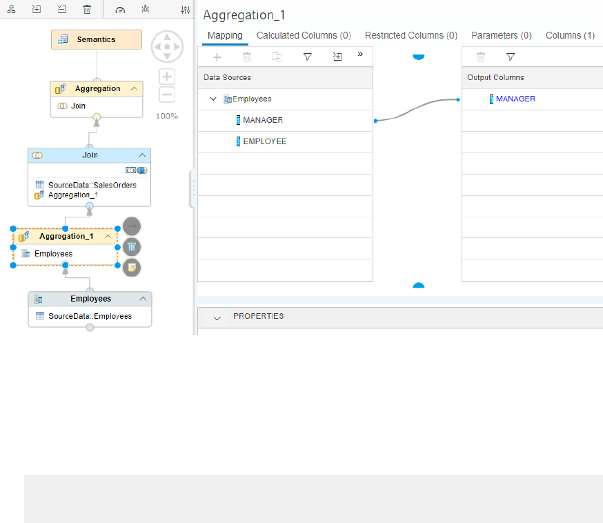
7.2.2.4.2 Example 2: Remodeling
Examples of remodeling include adding another eld, changing aggregations into projections, and so on.
Context
In the example below, the model rstly gives the same values for AMOUNT, irrespective of whether join pruning
occurs. After an additional eld is included with a keep ag, the AMOUNT for Alice and Hans changes,
depending on whether join pruning occurs.
Procedure
1. Use a copy of the previous calculation view and insert an aggregation node before the join. The aggregation
node maps only the MANAGER eld (therefore removing the EMPLOYEE eld):
When only the MANAGER eld is mapped in the aggregation node, multiple values for the same manager are
condensed into one value by the aggregation node.
2. Run the two SQL statements below. The rst statement allows join pruning to occur as it only requests
elds from the left table. The second statement prevents join pruning by also selecting the MANAGER eld
from the right table:
a. Query on elds from the left table only:
SELECT
"EMPLOYEE_1",
SUM("AMOUNT") AS "AMOUNT"
192
P U B L I C
SAP HANA Performance Guide for Developers
Optimization Features in Calculation Views
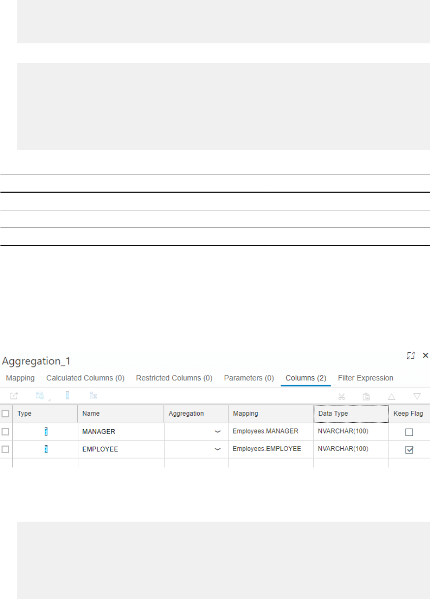
FROM
"JOINCARDINALITY_1"."joinCardinalityExample.db.CVs::joinCardinalityWrongAft
erRemodeling"
GROUP BY "EMPLOYEE_1"
b. Query on elds from both tables:
SELECT
"EMPLOYEE_1",
"MANAGER",
SUM("AMOUNT") AS "AMOUNT"
FROM
"JOINCARDINALITY_1"."joinCardinalityExample.db.CVs::joinCardinalityWrongAft
erRemodeling"
GROUP BY "EMPLOYEE_1","MANAGER"
Result: Query on Fields from the Left Table Only
Result: Query on Fields from Both Tables
EMPLOYEE_1 AMOUNT EMPLOYEE_1 MANAGER AMOUNT
Donald 20 Donald NULL 20
Alice 22 Alice Alice 22
Hans 40 Hans Hans 40
Horst 33 Horst NULL 33
As you can see, the values for AMOUNT are the same irrespective of whether join pruning occurs. The reason
is that the aggregation on the MANAGER join eld ensures that only distinct values enter the join from the
right. Your cardinality setting of 1..1 is therefore correct.
3. Now also map the EMPLOYEE eld in the aggregation node and set the Keep ag to make sure that the
EMPLOYEE eld is not pruned away if it is not requested:
4. Run the same queries again. Alice and Hans should now have dierent values for AMOUNT depending on
whether join pruning occurs:
a. Query on elds from the left table only:
SELECT
"EMPLOYEE_1",
SUM("AMOUNT") AS "AMOUNT"
FROM
"JOINCARDINALITY_1"."joinCardinalityExample.db.CVs::joinCardinalityWrongAft
erRemodeling"
GROUP BY "EMPLOYEE_1"
SAP HANA Performance Guide for Developers
Optimization Features in Calculation Views
P U B L I C 193
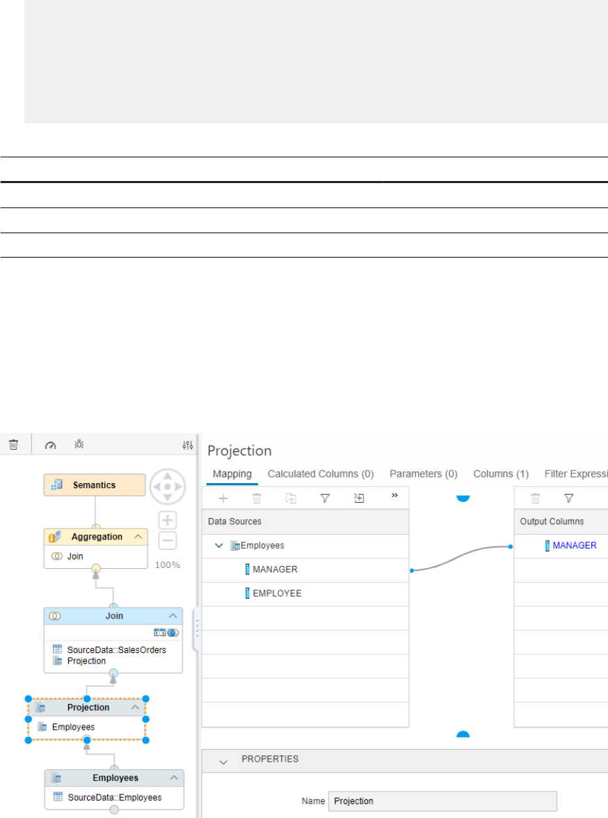
b. Query on elds from both tables:
SELECT
"EMPLOYEE_1",
"MANAGER",
SUM("AMOUNT") AS "AMOUNT"
FROM
"JOINCARDINALITY_1"."joinCardinalityExample.db.CVs::joinCardinalityWrongAft
erRemodeling"
GROUP BY "EMPLOYEE_1","MANAGER"
Result: Query on Fields from the Left Table Only
Result: Query on Fields from Both Tables
EMPLOYEE_1 AMOUNT EMPLOYEE_1 MANAGER AMOUNT
Donald 20 Donald NULL 20
Alice 22 Alice Alice 66
Hans 40 Hans Hans 80
Horst 33 Horst NULL 33
Dierent results occur when the EMPLOYEE eld is kept in the aggregation, leading to multiple occurrences
of the same value for the MANAGER eld.
This shows that a change to your model (adding another eld) below the join node might mean that your
right table entries are no longer unique when the join node is reached, which violates the cardinality
setting. Consequently, the values for AMOUNT depend on whether join pruning occurs.
5. Using the same calculation view, replace the aggregation with a projection:
When the aggregation node is changed to a projection node, the MANAGER eld no longer provides
exclusively distinct values to the join.
194
P U B L I C
SAP HANA Performance Guide for Developers
Optimization Features in Calculation Views

6. Run the two queries below and compare their results:
a. Query on elds from the left table only:
SELECT
"EMPLOYEE_1",
SUM("AMOUNT") AS "AMOUNT"
FROM
"JOINCARDINALITY_1"."joinCardinalityExample.db.CVs::joinCardinalityWrongAft
erRemodeling"
GROUP BY "EMPLOYEE_1"
b. Query on elds from both tables:
SELECT
"EMPLOYEE_1",
"MANAGER",
SUM("AMOUNT") AS "AMOUNT"
FROM
"JOINCARDINALITY_1"."joinCardinalityExample.db.CVs::joinCardinalityWrongAft
erRemodeling"
GROUP BY "EMPLOYEE_1","MANAGER"
Result: Query on Fields from the Left Table Only
Result: Query on Fields from Both Tables
EMPLOYEE_1 AMOUNT EMPLOYEE_1 MANAGER AMOUNT
Donald 20 Donald NULL 20
Alice 22 Alice Alice 66
Hans 40 Hans Hans 80
Horst 33 Horst NULL 33
As you can see, when the aggregation node is changed to a projection node, join pruning has an impact on
the resulting values for the AMOUNT measure. Therefore, any changes to the model below the join node,
such as changing an aggregation into a projection, might result in a violation of your join cardinality setting.
7.2.2.4.3 Example 3: Loading Additional Data
Like the second example, the third example also starts with a correct cardinality setting.
Procedure
1. Use the rst calculation view without any additional nodes, but replace the Employees table with a copy of
the table. A copy of the table is used so that it can be modied without inuencing the other models built
earlier:
SAP HANA Performance Guide for Developers
Optimization Features in Calculation Views
P U B L I C 195
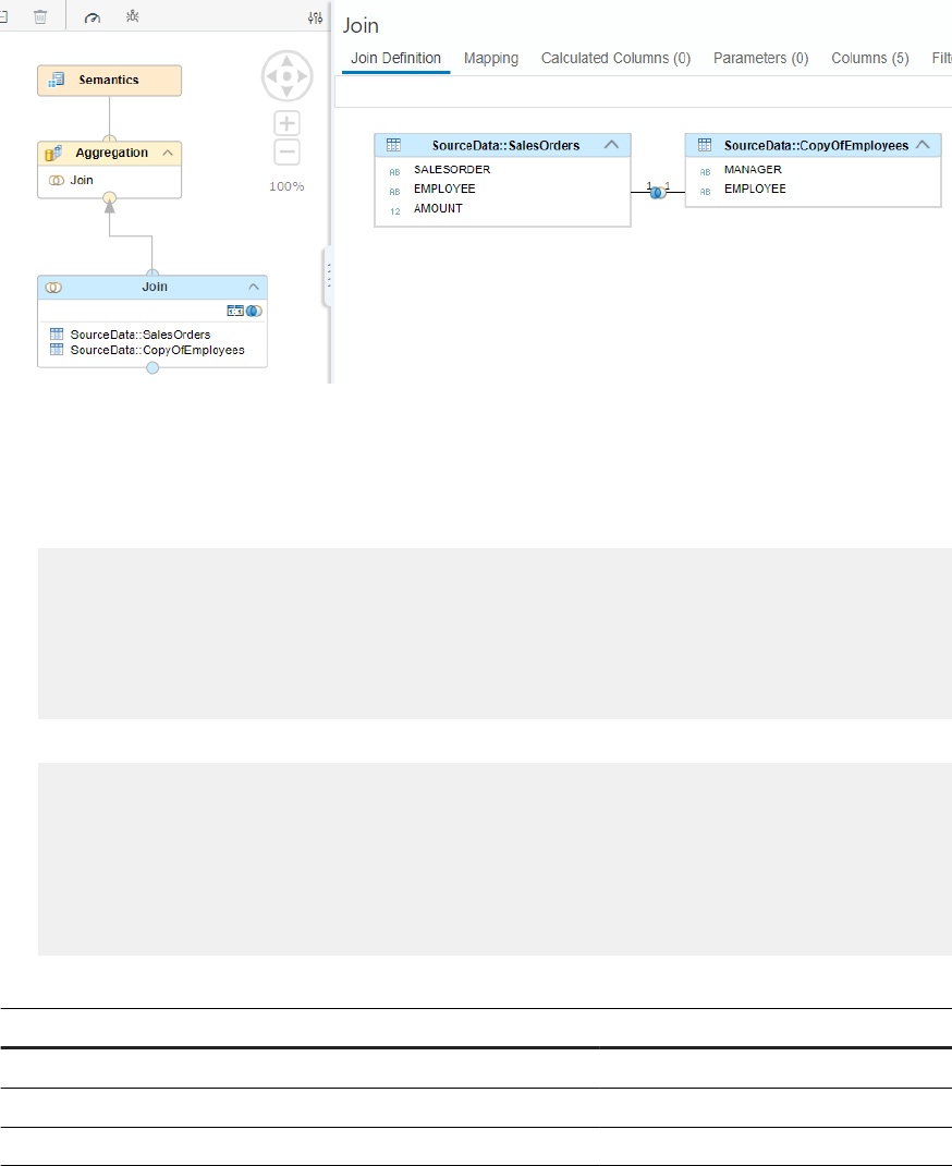
The join is dened on the EMPLOYEE eld on both sides and the cardinality setting of 1..1 reects the true
data cardinality. Now also query the EMPLOYEE eld in the right table to check the impact of join pruning.
2. Run the two queries below and compare their results:
a. Query on elds from the left table only:
SELECT
"EMPLOYEE_1",
SUM("AMOUNT") AS "AMOUNT"
FROM
"JOINCARDINALITY_1"."joinCardinalityExample.db.CVs::joinCardinalityWrongAft
erLoading"
GROUP BY "EMPLOYEE_1"
b. Query on elds from both tables:
SELECT
"EMPLOYEE_1",
"EMPLOYEE",
SUM("AMOUNT") AS "AMOUNT"
FROM
"JOINCARDINALITY_1"."joinCardinalityExample.db.CVs::joinCardinalityWrongAft
erLoading"
GROUP BY "EMPLOYEE_1","EMPLOYEE"
Result: Query on Fields from the Left Table Only
Result: Query on Fields from Both Tables
EMPLOYEE_1 AMOUNT EMPLOYEE_1 MANAGER AMOUNT
Donald 20 Donald Donald 20
Alice 22 Alice Alice 22
Hans 40 Hans Hans 40
Horst 33 Horst Horst 33
As expected, when the cardinality setting in the calculation view reects the data cardinality, the same
values are returned for AMOUNT, irrespective of whether join pruning occurs.
3. Imagine that Donald gets a second manager, Herbert, and add this record to the CopyOfEmployees table:
196
P U B L I C
SAP HANA Performance Guide for Developers
Optimization Features in Calculation Views

MANAGER EMPLOYEE
null Alice
Alice Donald
Alice Dagobert
Alice Hans
Hans Heinz
Hans Jane
? Horst
Herbert Donald
Due to this change, your cardinality setting of 1..1 for the EMPLOYEE eld is no longer reected in the
data. Consequently, you will see dierent values for Donald’s AMOUNT, depending on whether the join is
executed.
4. Run the two queries below and compare their results:
a. Query on elds from the left table only:
SELECT
"EMPLOYEE_1",
SUM("AMOUNT") AS "AMOUNT"
FROM
"JOINCARDINALITY_1"."joinCardinalityExample.db.CVs::joinCardinalityWrongAft
erLoading"
GROUP BY "EMPLOYEE_1"
b. Query on elds from both tables:
SELECT
"EMPLOYEE_1",
"EMPLOYEE",
SUM("AMOUNT") AS "AMOUNT"
FROM
"JOINCARDINALITY_1"."joinCardinalityExample.db.CVs::joinCardinalityWrongAft
erLoading"
GROUP BY "EMPLOYEE_1","EMPLOYEE"
Result: Query on Fields from the Left Table Only
Result: Query on Fields from Both Tables
EMPLOYEE_1 AMOUNT EMPLOYEE_1 MANAGER AMOUNT
Donald 20 Donald Donald 40
Alice 22 Alice Alice 22
Hans 40 Hans Hans 40
Horst 33 Horst Horst 33
As shown above, inconsistent results are returned when additional data leads to a dierence between the
cardinality setting and the data cardinality. Donald’s AMOUNT varies depending on whether the join is
executed. This is a consequence of the cardinality setting, which was initially correct, but became incorrect
after additional data was loaded.
SAP HANA Performance Guide for Developers
Optimization Features in Calculation Views
P U B L I C 197
7.3 Optimizing Join Columns
By explicitly allowing join columns to be optimized, you can potentially reduce the number of records that need
to be processed at later stages of query processing, resulting in better performance and reduced resource
consumption.
This is because aggregation can then occur at an earlier stage of query processing, which allows the number of
records to be reduced early on. This is particularly relevant in scenarios in which there are many joins dened
on dierent elds, but the columns requested by the query are from just a few of the join partners. In these
cases, taking the join eld out of the aggregation level might allow the number of records that need to be
processed further to be signicantly reduced.
Note this is not the default query behavior, because when columns are removed, the aggregation behavior of
the query could be changed, which could lead to measures having dierent resulting values. Therefore, by
default, all columns on which joins are dened are requested during query processing, irrespective of whether
they are required by the query, to ensure consistent aggregation behavior.
7.3.1 Optimize Join Columns Option
There may be cases where join columns can be omitted. Consider a scenario in which a query requests elds
from only one join partner, the cardinality to the other join partner (from which none of the elds are
requested) is set to 1, and the join is not an inner join.
In this case, executing the join does not aect the result. Since the join does not have to be executed and the
join eld has not been requested by the query, it is a candidate for pruning. By default, it will not be pruned, but
if the Optimize Join Columns option is set, it can be removed.
In cases where there are multiple join partners on dierent join elds and where queries typically only select
elds from a small subset of join partners, the Optimize Join Columns option can be used to allow various join
elds to be excluded from the aggregation. This is because the option explicitly states that the join elds do not
have to be included in the aggregation. By omitting the join eld and thus omitting a eld that might otherwise
increase the granularity of the aggregation, the number of records that need to be further processed can be
signicantly reduced. As a result, better performance and lower memory consumption can be achieved. The
extent of improvement depends on which elds the queries request at runtime and on which elds the joins are
dened.
However, when using the Optimize Join Columns option, you should be aware of the following side eects:
● An incorrect cardinality setting might lead to the wrong result, from your perspective (technically, the
optimizer has behaved correctly). The use of the Optimize Join Columns option requires that the cardinality
is set correctly (see the prerequisites in this section).
● When the Optimize Join Columns option is set, the optimizer changes the aggregation level by excluding
the join column from the aggregation, if possible. Whether the join column can be excluded also depends
on which elds are queried. This means that the inclusion or exclusion of the join column in the aggregation
level varies depending on the elds that are requested by the query. If you have aggregation functions for
which the aggregation level matters (such as nding the maximum), the results can change depending on
the aggregation level. This is demonstrated by the example in this section.
198
P U B L I C
SAP HANA Performance Guide for Developers
Optimization Features in Calculation Views

7.3.2 Prerequisites for Pruning Join Columns
Join column pruning can only occur if all the following conditions are met:
● The join eld is not requested by the query.
● Only elds from one of the join partners are requested by the query.
● The join is either an outer join, referential join, or text join.
● The cardinality to the join partner from which none of the elds are requested is set to 1.
The reasons for these prerequisites are as follows:
● If a join eld is requested by the query, it cannot simply be excluded.
● If elds are requested from both join partners, the join must be executed and therefore the join eld must
be requested.
● If the join is not an outer, referential, or text join, the join might add or delete records. The example (below)
shows the dierence between inner and outer joins in terms of preserving the number of records.
● If the table to be pruned might deliver more than one matching partner, join pruning should not occur.
Therefore, the cardinality of the table that does not deliver any elds needs to be set to 1. However, the
optimizer does not check at runtime whether more than one matching partner could occur, so it is your
responsibility to ensure that your cardinality setting of 1 reects the actual data cardinality.
Example: The eect of inner joins and outer joins on the number of records
The example below shows the dierence between inner and outer joins in terms of preserving the number of
records.
Table 1 has the following entries in its join eld:
a,b,c
Table 2 has the following entries in its join eld:
a,a,a,b
You can create the tables as follows:
create column table leftTable (joinField NVARCHAR(10), measure Int);
create column table rightTable (joinField NVARCHAR(10));
insert into leftTable values ('a',10);
insert into leftTable values ('b',20);
insert into leftTable values ('c',30);
insert into rightTable values ('a');
insert into rightTable values ('a');
insert into rightTable values ('a');
insert into rightTable values ('b');
Inner join
When an inner join is used, only the entries that have a matching partner are retrieved.
Run the following query:
select
SAP HANA Performance Guide for Developers
Optimization Features in Calculation Views
P U B L I C 199

l.joinfield "leftJoinfield",
l.measure "measure",
r.joinfield "rightJoinfield"
from
leftTable l
inner join
rightTable r
on
l.joinField=r.joinField
The output is as follows:
leftJoinField
measure rightJoinField
a 10 a
a 10 a
a 10 a
b 20 b
The output contains the entries a,a,a,b from table 1. The record with the value a from table 1 is tripled
because there are three matching entries in table 2. The entry c is omitted because there are no matching
entries in table 2.
This shows that an inner join can result in a changed number of output records depending on whether the join
is executed. In this example, the number of output records in the left table changes from 3 to 4, but this
number could be higher or lower depending on the entries in the right table.
Outer join
When an outer join is used, entries without a matching entry in the right table are retrieved as well.
Run the following query:
select
l.joinfield "leftJoinfield",
l.measure "measure",
r.joinfield "rightJoinfield"
from
leftTable l
left outer join
rightTable r
on
l.joinField=r.joinField
This time the output is as follows:
leftJoinField
measure rightJoinField
a 10 a
a 10 a
a 10 a
b 20 b
c 30 ?
You can see that the entry c is not omitted even though there is no match in the right table. To this extent, outer
joins preserve the number of output records. However, you can also see that the entry
a has once again been
200
P U B L I C
SAP HANA Performance Guide for Developers
Optimization Features in Calculation Views

tripled. This means that the number of output records can change if there is more than one matching entry in
the right table. Therefore, it is important to ensure that the correct cardinality is specied (the fourth
prerequisite above).
By setting the cardinality, for example, to n:1 so that there is at most one match in the right table, entries will
not be duplicated when the join is executed because every entry in the left table has at most one entry in the
right table. If an entry in the left table does not have a matching entry in the right table, this is not a problem,
because the value will still be kept, as can be seen in the case of entry c above.
This means that when a cardinality of 1 is set for the right table, the execution of the join does not inuence the
number of records that are processed further, and the join can therefore be omitted if there are no elds that
must be read from the right table.
Note that if you use the wrong cardinality, the output might be incorrect because pruning of the join might
occur even though the join would inuence the number of records returned for further processing.
7.3.3 Example
This example shows the impact of the Optimize Join Columns option on query processing. In the example, a
simple calculation view is modeled rstly with the Optimize Join Columns option set, and secondly without it
set.
The debug mode is used to check that join pruning occurs and that the intermediate aggregation level is
changed when the option is set. In addition, an aggregation function is used that is aected by the level of
aggregation. It is used to demonstrate how the elds requested in the query can change the resulting values of
the measures.
The example consists of the following steps:
1. Create the Tables [page 201]
2. Create the Calculation View [page 202]
3. Run the Queries [page 205]
4. Debug the Queries [page 206]
5. Analyze the Queries [page 209]
6. Change the Requested Fields [page 210]
7.3.3.1 Create the Tables
Create the tables needed for this example.
ItemsMD
ITEM DESCRIPTION
001 Diapers
002 Diapers
003 Milk
SAP HANA Performance Guide for Developers
Optimization Features in Calculation Views
P U B L I C 201
ItemsMD
ITEM DESCRIPTION
004 Wine
Sample Code
INSERT INTO "ItemsMD" VALUES ('001','Diapers');
INSERT INTO "ItemsMD" VALUES ('002','Diapers');
INSERT INTO "ItemsMD" VALUES ('003','Milk');
INSERT INTO "ItemsMD" VALUES ('004','Wine');
SalesItems
ITEM EMPLOYEE AMOUNT
001 Donald 10
002 Donald 50
003 Alice 40
004 Dagobert 21
Sample Code
INSERT INTO "SalesItems" VALUES ('001','Donald',10);
INSERT INTO "SalesItems" VALUES ('002','Donald',50);
INSERT INTO "SalesItems" VALUES ('003','Alice',40);
INSERT INTO "SalesItems" VALUES ('004','Dagobert',21);
7.3.3.2 Create the Calculation View
Create the calculation view needed for this example.
Procedure
1. Create a calculation view:
a. Add an aggregation node and then add the SalesItems table to it as a data source.
b. Map all columns to the output and select the aggregation type MAX for the AMOUNT column.
202
P U B L I C
SAP HANA Performance Guide for Developers
Optimization Features in Calculation Views

The calculation view should now look like this:
2. Add a join node:
a. Connect the join node to both aggregation nodes.
b. Join the ItemsMD table on the ITEM column with a left-outer join. Use the aggregation node as the left
join partner
c. Keep the cardinality setting n..m.
d. Select the Optimize Join Columns checkbox.
The view should not look like this:
3. Map all columns to the output except the ITEM column from the ItemsMD table.
4. In the higher-level aggregation node, map all columns to the output
5. In the semantics node, change the aggregation type of the AMOUNT column to SUM:
SAP HANA Performance Guide for Developers
Optimization Features in Calculation Views
P U B L I C 203
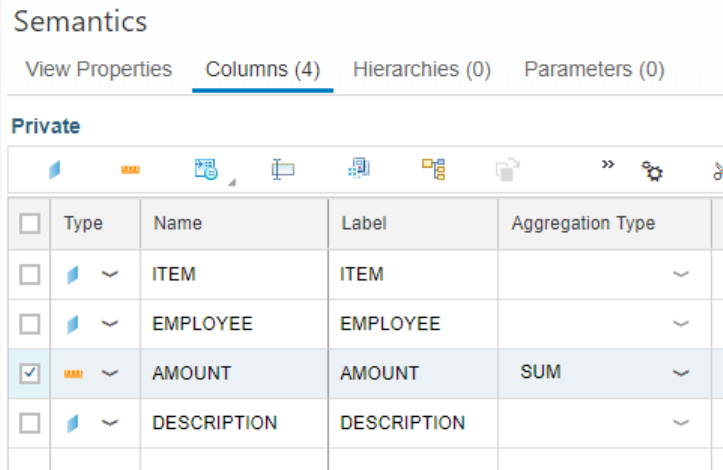
6. Try to build the calculation view.
The build will fail. You will see an error message stating that you need a cardinality setting of N:1 or 1:1 when
using the Optimize Join Columns option. This tells you that not all prerequisites for the Optimize Join
Columns option have been met. The n..m cardinality setting has therefore prevented join pruning from
occurring.
7. Set the cardinality to n:1. As a best practice, check that this cardinality reects the data cardinality and
that there is never more than one matching entry for the join column item in the right table. In a real
scenario, you might want to enforce this by applying some underlying loading logic.
204
P U B L I C
SAP HANA Performance Guide for Developers
Optimization Features in Calculation Views
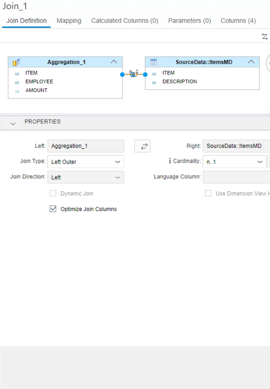
8. Build the view again.
7.3.3.3 Run the Queries
Test the calculation view by running the queries below with and without the Optimize Join Columns option set.
Procedure
1. With the Optimize Join Columns option still selected, run the following query, which requests elds from
SalesItem table only:
SELECT
"EMPLOYEE",
SUM("AMOUNT") AS "AMOUNT"
FROM
"OPTIMIZEJOINCOLUMN_HDI_DB_1"."exampleOptimizeJoinColumns"
GROUP BY "EMPLOYEE"
You should see the following output:
SAP HANA Performance Guide for Developers
Optimization Features in Calculation Views
P U B L I C 205

EMPLOYEE AMOUNT
Donald 50
Alice 40
Dagobert 21
2. Deselect the Optimize Join Columns option and build the view again.
3. Run the same query as above.
You should see dierent results:
EMPLOYEE
AMOUNT
Donald 60
Alice 40
Dagobert 21
Results
As you can see, the amount for Donald diers depending on whether the Optimize Join Columns option is set.
The reason for this is that in the rst query the join eld ITEM is excluded (pruned) because the prerequisites
outlined above are met:
● The join eld ITEM is not requested by the query.
● Only the elds from one join partner are requested; the only elds requested are EMPLOYEE and AMOUNT
and they both come from the left table.
● The join is a left outer join.
● The cardinality to the join partner from which none of the elds are requested was set to 1.
The pruning of the join eld ITEM changes the aggregation level for the maximum calculation that was dened
in the aggregation node.
7.3.3.4 Debug the Queries
For a better understanding of why the values changed, run the queries above in debug mode.
Procedure
1. Open the calculation view. The Optimize Join Columns option should still be deselected. To start
debugging, select the Semantics node and then choose the Debug button.
2. Replace the default query with the query previously used:
SELECT
206
P U B L I C
SAP HANA Performance Guide for Developers
Optimization Features in Calculation Views
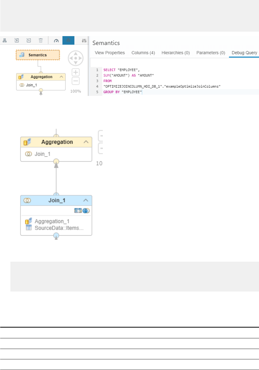
"EMPLOYEE",
SUM("AMOUNT") AS "AMOUNT"
FROM
"OPTIMIZEJOINCOLUMN_HDI_DB_1"."exampleOptimizeJoinColumns"
GROUP BY "EMPLOYEE"
3. Click Execute to run the query.
You should see the following:
○ The join node is grayed out. This indicates that join pruning has occurred:
○ The debug query of the lower-level aggregation node contains the ITEM column even though ITEM was
not requested in the end-user query:
SELECT "EMPLOYEE", "ITEM", "AMOUNT" FROM
"OPTIMIZEJOINCOLUMN_HDI_DB_1"."exampleOptimizeJoinColumns/dp
/Aggregation_1"('PLACEHOLDER'=('$$client$$','$$client$$'),
'PLACEHOLDER'=('$$language$$','$$language$$'))
4. Execute the debug query of the lower-level aggregation node.
You should see the following intermediate values:
EMPLOYEE
ITEM AMOUNT
Donald 001 10
Donald 002 50
Alice 003 40
Dagobert 004 21
5. Exit the debug session, select the Optimize Join Columns option, and build the calculation view again.
SAP HANA Performance Guide for Developers
Optimization Features in Calculation Views
P U B L I C 207

6. Start the debug session as described above and execute the same debug query:
SELECT
"EMPLOYEE",
SUM("AMOUNT") AS "AMOUNT"
FROM
"OPTIMIZEJOINCOLUMN_HDI_DB_1"."exampleOptimizeJoinColumns"
GROUP BY "EMPLOYEE"
You should see the following:
○ Like before, the join node is grayed out. This indicates that join pruning has occurred.
○ This time the debug query of the lower-level aggregation node does not contain the ITEM column. This
shows that the
Optimize Join Columns feature excludes the ITEM join column at an early stage of
processing.
7. Execute the debug query of the lower-level aggregation node.
You should see the following intermediate values:
EMPLOYEE
AMOUNT
Donald 50
Alice 40
Dagobert 21
Results
The maximum values are calculated based on the intermediate values of the lower-level aggregation node.
When the Optimize Join Columns option is not selected, the ITEM column is kept in the aggregation granularity
and the maximum calculation therefore involves both of Donald's records (item 001 and 002), leading to
max(10)+max(50)=60. The summing stems from the fact that you selected the aggregation mode SUM in the
semantics node. In contrast, when the Optimize Join Columns option is selected, just one record is calculated
for Donald: max(10,50)=50.
You therefore see dierent results for Donald, depending on whether the join column is omitted. If you had not
used MAX as the aggregation function but, for example, SUM, in the aggregation node, you would not see the
impact of join column pruning. This is because SUM is not sensitive to the aggregation level on which it is
calculated.
Note that you see fewer records at the intermediate nodes when the Optimize Join Columns option is set
compared to when it is not set (3 versus 4 records in this example). In this example, the impact is small, but if
you have many join elds that could be pruned and the join elds also have high cardinalities, pruning might
have a substantial impact on the level of aggregation and thus the number of records that need to be processed
further. This means that performance benets can be achieved when the Optimize Join Columns option is used
correctly.
208
P U B L I C
SAP HANA Performance Guide for Developers
Optimization Features in Calculation Views
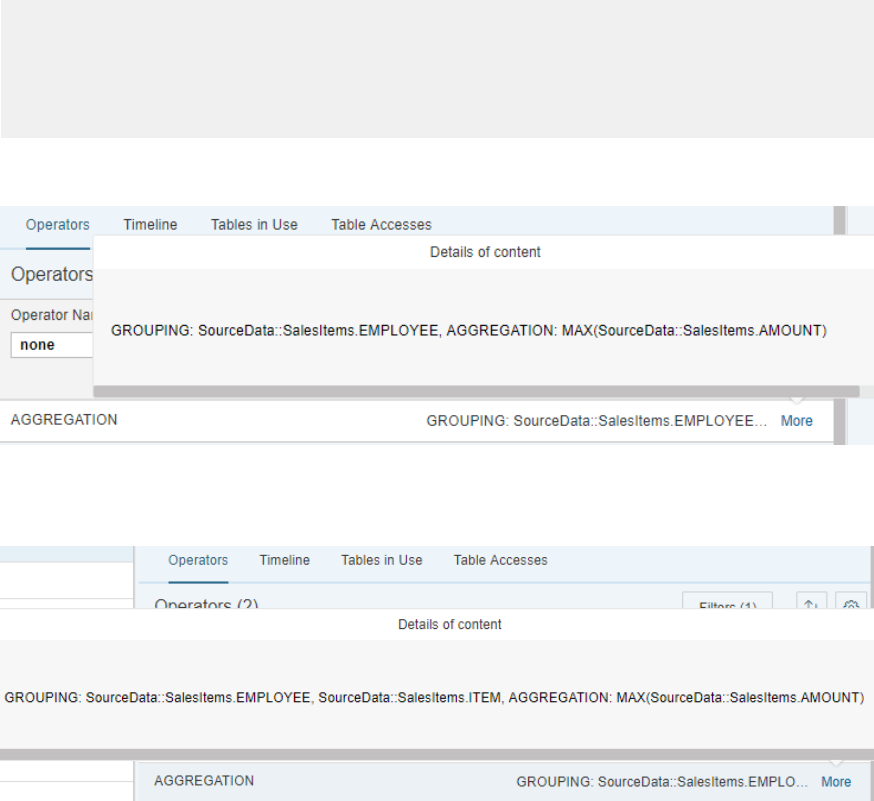
7.3.3.5 Analyze the Queries
You can use the Database Explorer to run the queries above in SQL analysis mode and check whether the join
eld is omitted.
Procedure
1. Firstly check the calculation view with the Optimize Join Columns option selected. To do so, open an SQL
console and enter the query to be run. For example:
SELECT
"EMPLOYEE",
SUM("AMOUNT") AS "AMOUNT"
FROM
"OPTIMIZEJOINCOLUMN_HDI_DB_1"."exampleOptimizeJoinColumns"
GROUP BY "EMPLOYEE"
2. From the Run dropdown menu, choose Analyze SQL.
3. On the Operators tab, check the Aggregation details. For example:
4. Repeat the steps above on the same calculation view but this time without the Optimize Join Columns
option set.
5. Again, on the Operators tab, check the Aggregation details. For example:
Results
The query on the calculation view with the Optimize Join Columns option set does not contain the ITEM eld in
the aggregation level. However, the query on the calculation view without the Optimize Join Columns option set
SAP HANA Performance Guide for Developers
Optimization Features in Calculation Views
P U B L I C 209

does contain the ITEM eld in the grouping. Therefore, as this example conrms, join column pruning has been
eective.
7.3.3.6 Change the Requested Fields
Finally, to demonstrate how join column pruning can change the resulting measure values depending on the
elds requested, request one of the elds (in this example, DESCRIPTION) from the right table so that join
pruning and therefore join column pruning cannot occur.
Procedure
Run the following query with the Optimize Join Columns option set:
SELECT
"DESCRIPTION",
"EMPLOYEE",
SUM("AMOUNT") AS "AMOUNT"
FROM
"OPTIMIZEJOINCOLUMN_HDI_DB_1"."exampleOptimizeJoinColumns"
GROUP BY "DESCRIPTION"",EMPLOYEE"
Result: Query with the DESCRIPTION Field
Result: Query without the DESCRIPTION Field
DESCRIPTION EMPLOYEE AMOUNT EMPLOYEE AMOUNT
Diapers Donald 60 Donald 50
Wine Dagobert 21 Alice 40
Milk Alice 40 Dagobert 21
As you can see, the results are dierent when the additional column is requested from the right table and the
Optimize Join Columns option is set.
7.4 Using Dynamic Joins
Dynamic joins help improve the join execution process by reducing the number of records processed by the join
view node at runtime.
A dynamic join is a special join that comprises more than one join eld. Which elds are evaluated at runtime is
determined based on the requested elds. For example, Table1 and Table2 are joined on Field1 and Field2.
However, when only Field1 or only Field2 is requested by the client, the tables (Table1 and Table2) are joined
based only on the requested eld (Field1 or Field2).
This is dierent from the classical join behavior. In the classical join, the join condition is static, meaning that
the join condition does not change according to the client query. In the case of the dynamic join, on the other
hand, the join condition changes dynamically based on the query.
210
P U B L I C
SAP HANA Performance Guide for Developers
Optimization Features in Calculation Views

This dierence in behavior can lead to dierences in the query result sets, so it is important to understand the
implications of using the dynamic join before applying it.
Note that to use dynamic joins, at least one of the elds involved in the join condition must be contained in the
requested list of elds of the query. If that is not the case, a query runtime error will occur.
7.4.1 Dynamic Join Example
This simple example shows the eect of the dynamic join and how it diers from the classical join. In this
example, you are evaluating material sales data and want to calculate the sales share of a material.
Dataset
The dataset shown below contains the material sales data for materials at region and country level:
DynamicSalesShare
REGION COUNTRY MATERIAL SALES
APJ CHN PROD1 10
APJ CHN PROD2 10
APJ CHN PROD3 0
APJ IND PROD1 20
APJ IND PROD2 50
APJ IND PROD3 60
EUR DE PROD1 50
EUR DE PROD2 100
EUR DE PROD3 60
EUR UK PROD1 20
EUR UK PROD2 30
EUR UK PROD3 40
SAP HANA Performance Guide for Developers
Optimization Features in Calculation Views
P U B L I C 211
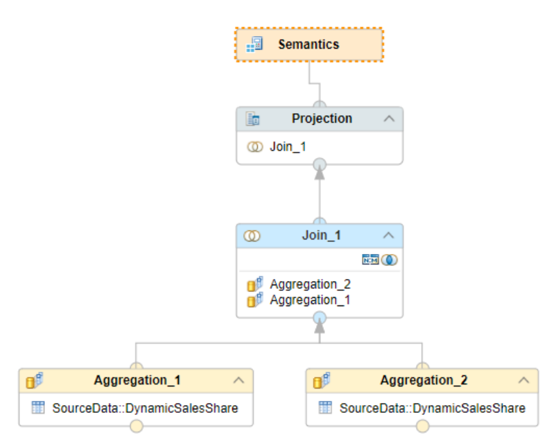
Model with a Dynamic Join
In the model below, the dataset shown above is joined using two aggregation nodes (both with the data source
DynamicSalesShare):
212 P U B L I C
SAP HANA Performance Guide for Developers
Optimization Features in Calculation Views
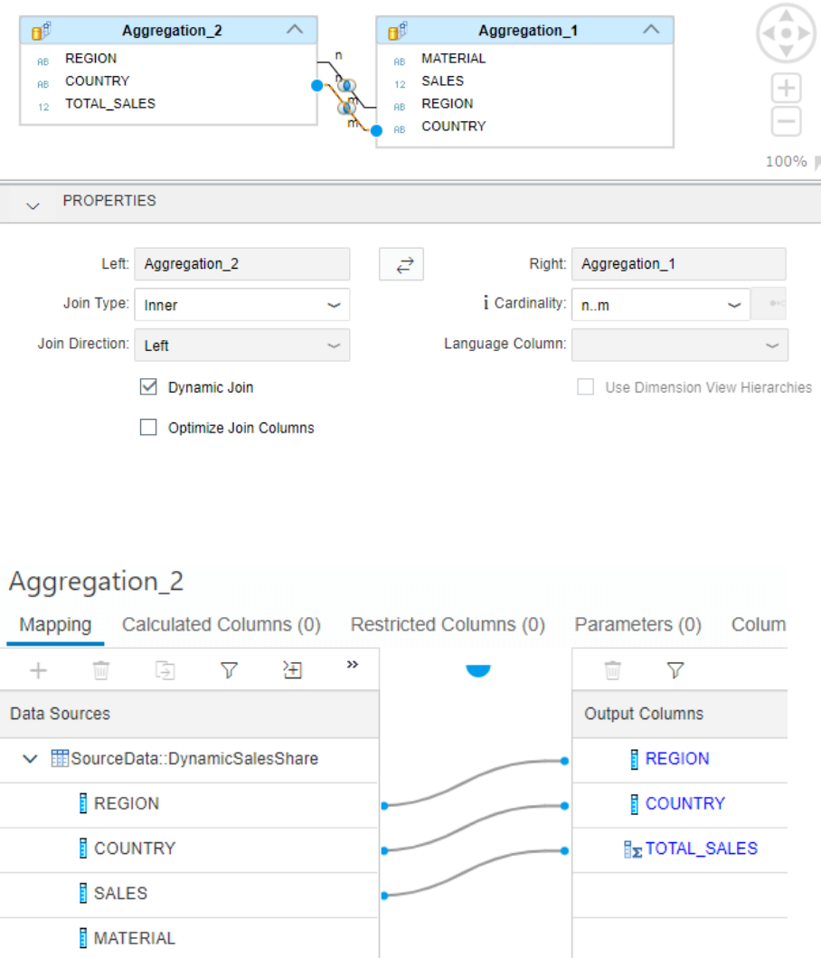
Dynamic Join
The two aggregation nodes are joined dynamically on the elds REGION and COUNTRY:
Total Sales
The aggregation node on the right (Aggregation_2) does not contain the Material eld as one of its output
columns. Therefore, this node always returns the total sales of a given region or country:
SAP HANA Performance Guide for Developers
Optimization Features in Calculation Views
P U B L I C 213
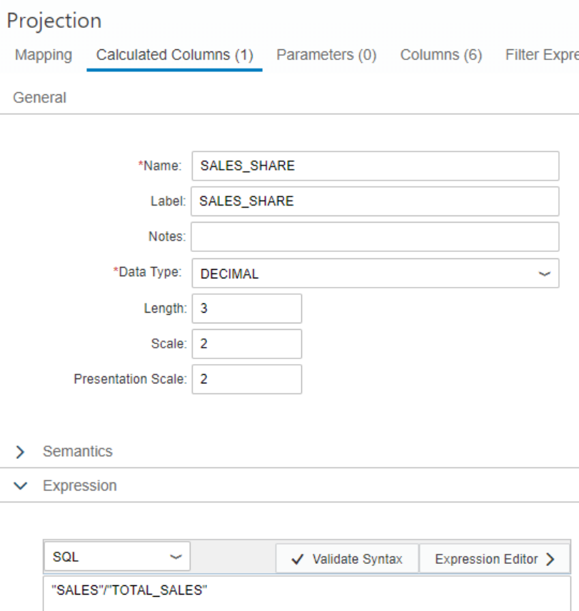
Sales Share
The sales share is dened as a calculated column in the projection node:
Model with a Classical Join
You can build a similar model to the one above using a classical join on the elds REGION and COUNTRY.
Queries
The following SELECT statements illustrate the dierence in the join logic of the two joins and the resulting
dierence in the query result.
214
P U B L I C
SAP HANA Performance Guide for Developers
Optimization Features in Calculation Views

Queries at Country Level
The simple query on the models evaluates the sales share of the materials at country level.
Query on the model with the dynamic join:
SELECT "COUNTRY","MATERIAL",SUM("SALES"),SUM("TOTAL_SALES"),SUM("SALES_SHARE")
FROM
"JOINCARDINALITY_1"."joinCardinalityExample.db.CVs::TestDynamicJoin"
GROUP BY "COUNTRY","MATERIAL"
ORDER BY "COUNTRY","MATERIAL";
COUNTRY
MATERIAL SUM(SALES) SUM(TOTAL_SALES) SUM(SALES_SHARE)
CHN PROD1 10 20 0.5
CHN PROD2 10 20 0.5
CHN PROD3 0 20 0
IND PROD1 50 210 0.23
IND PROD2 100 210 0.47
IND PROD3 60 210 0.28
DE PROD1 20 130 0.15
DE PROD2 50 130 0.38
DE PROD3 60 130 0.46
UK PROD1 20 90 0.22
UK PROD2 30 90 0.33
UK PROD3 40 90 0.44
Query on the model with the classical join:
SELECT "COUNTRY","MATERIAL",SUM("SALES"),SUM("TOTAL_SALES"),SUM("SALES_SHARE")
FROM
"JOINCARDINALITY_1"."joinCardinalityExample.db.CVs::TestStaticJoin"
GROUP BY "COUNTRY","MATERIAL"
ORDER BY "COUNTRY","MATERIAL";
COUNTRY
MATERIAL SUM(SALES) SUM(TOTAL_SALES) SUM(SALES_SHARE)
CHN PROD1 10 20 0.5
CHN PROD2 10 20 0.5
CHN PROD3 0 20 0
IND PROD1 50 210 0.23
IND PROD2 100 210 0.47
IND PROD3 60 210 0.28
DE PROD1 20 130 0.15
DE PROD2 50 130 0.38
DE PROD3 60 130 0.46
UK PROD1 20 90 0.22
SAP HANA Performance Guide for Developers
Optimization Features in Calculation Views
P U B L I C 215
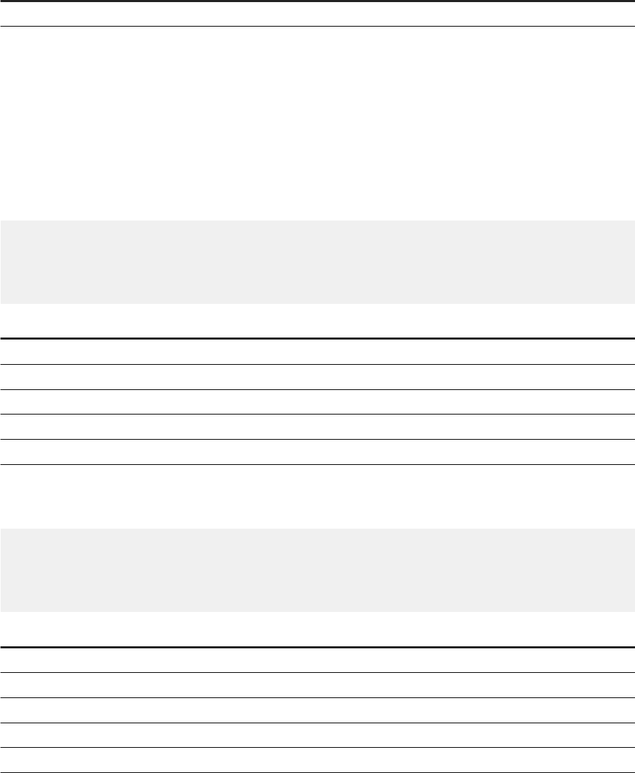
COUNTRY MATERIAL SUM(SALES) SUM(TOTAL_SALES) SUM(SALES_SHARE)
UK PROD2 30 90 0.33
UK PROD3 40 90 0.44
As can be seen, the result set of both queries are identical irrespective of the join type (dynamic or classical).
Queries at Region Level
When the query is changed to evaluate the sales share at region level (which is basically a higher aggregation
level than country), the dierence becomes apparent. The result sets showing the sales share of materials per
region are as follows.
Query on the model with the dynamic join:
SELECT "REGION","MATERIAL",SUM("SALES"),SUM("TOTAL_SALES"),SUM("SALES_SHARE")
FROM
"JOINCARDINALITY_1"."joinCardinalityExample.db.CVs::TestDynamicJoin"
GROUP BY "REGION","MATERIAL"
ORDER BY "REGION","MATERIAL";
REGION
MATERIAL SUM(SALES) SUM(TOTAL_SALES) SUM(SALES_SHARE)
APJ PROD1 30 150 0.2
APJ PROD2 60 150 0.4
APJ PROD3 60 150 0.4
EUR PROD1 70 300 0.23
EUR PROD2 130 300 0.43
EUR PROD3 100 300 0.33
Query on the model with the classical join:
SELECT "REGION","MATERIAL",SUM("SALES"),SUM("TOTAL_SALES"),SUM("SALES_SHARE")
FROM
"JOINCARDINALITY_1"."joinCardinalityExample.db.CVs::TestStaticJoin"
GROUP BY "REGION","MATERIAL"
ORDER BY "REGION","MATERIAL";
REGION
MATERIAL SUM(SALES) SUM(TOTAL_SALES) SUM(SALES_SHARE)
APJ PROD1 30 150 0.65
APJ PROD2 60 150 0.88
APJ PROD3 60 150 0.46
EUR PROD1 70 300 0.46
EUR PROD2 130 300 0.8
EUR PROD3 100 300 0.73
As can be seen, the dynamic join returns the sales share at region level by aggregating the sales value before
joining the datasets. The classical join model, however, rst calculates the sales share at region plus country
level (because the join condition contains both region and country) and then aggregates the resulting sales
share after the join has been executed.
216
P U B L I C
SAP HANA Performance Guide for Developers
Optimization Features in Calculation Views

7.4.2 Workaround for Queries Without Requested Join
Attributes
As mentioned above, a query on a calculation view with a dynamic join results in an error when none of the
columns involved in the join are requested.
Context
The example below shows a typical error:
Output Code
Could not execute 'SELECT SUM("SALES"),SUM("TOTAL_SALES"),SUM("SALES_SHARE")
FROM …'
Error: (dberror) [2048]: column store error: search table error: [34023]
Instantiation of calculation model failed;exception 306116:
At least one join attribute of the dynamic join should be requested on node
'Join_1'
To handle situations where a model could be queried without any join-relevant columns in the drilldown (in
other words, in the GROUP BY clause), the model depicted earlier can be enhanced with a DUMMY column, as
described below.
Procedure
1. Add a calculated column (called DUMMY) to the aggregation nodes on both sides of the join. The column
contains a constant value:
SAP HANA Performance Guide for Developers
Optimization Features in Calculation Views
P U B L I C 217
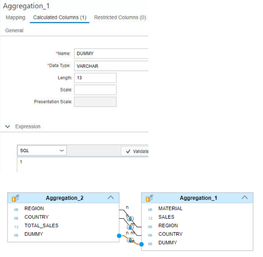
2. Include the DUMMY columns in the join condition:
3. In the output projection node, set the Keep Flag option on the DUMMY column to ensure that the DUMMY
column is always contained in the drilldown, even if it is not explicitly requested:
218
P U B L I C
SAP HANA Performance Guide for Developers
Optimization Features in Calculation Views
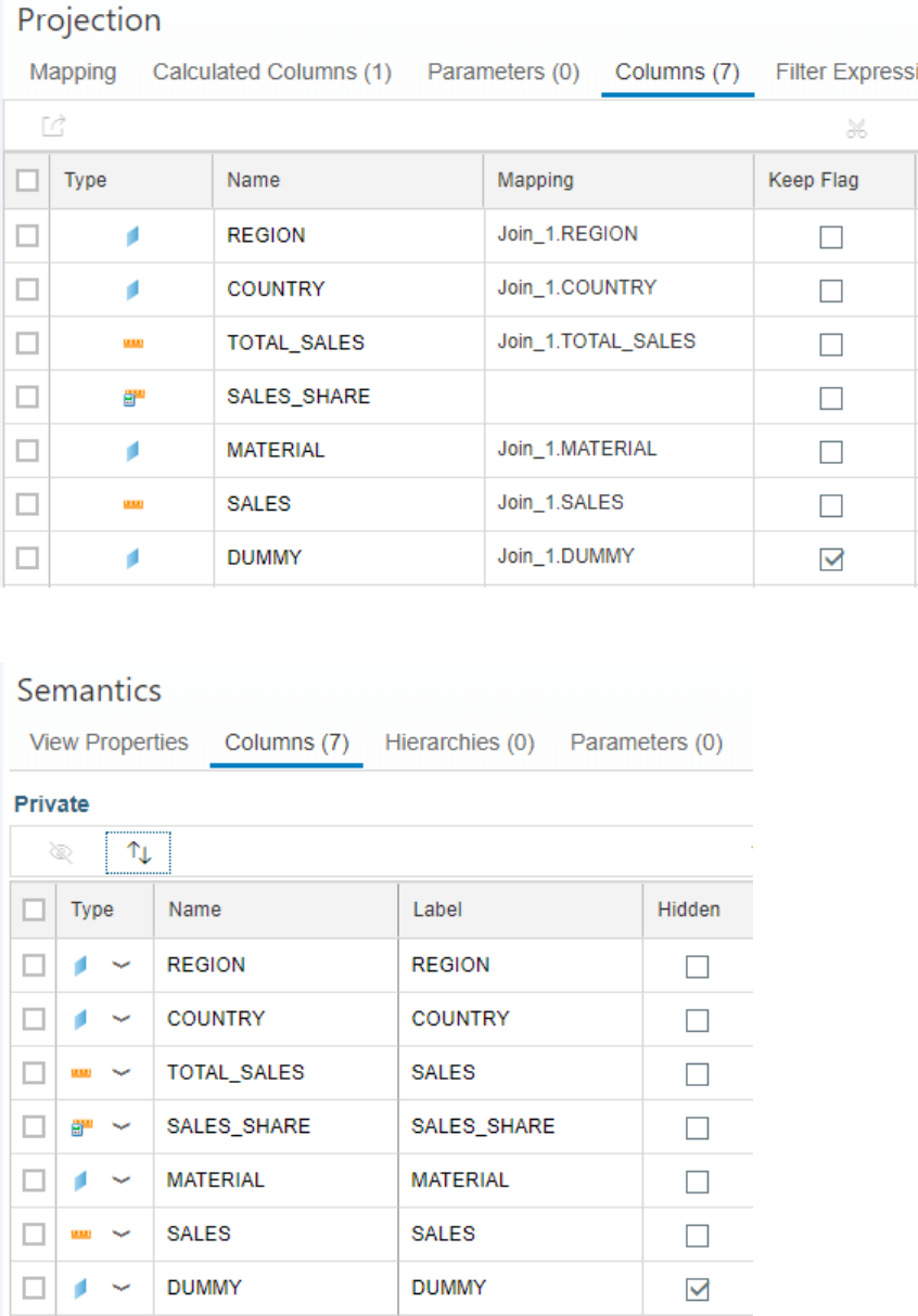
4. In the semantics node, set the DUMMY column to Hidden to avoid confusion when the calculation view is
used (the DUMMY column has been created purely for technical reasons):
SAP HANA Performance Guide for Developers
Optimization Features in Calculation Views
P U B L I C 219

5. Execute the same query that previously resulted in an error, as shown below:
SELECT SUM("SALES"),SUM("TOTAL_SALES"),SUM("SALES_SHARE")
FROM
"JOINCARDINALITY_1"."joinCardinalityExample.db.CVs::TestDynamicJoinNoAttribute
s";
SUM(SALES) SUM(TOTAL_SALES) SUM(SALES_SHARE)
450 450 1
7.5 Union Node Pruning
Union node pruning allows the data sources in union nodes to be pruned. It is based on dened criteria that at
runtime exclude specic data sources from the processing. This helps reduce resource consumption and
benets performance.
To prune data sources, you need either a pruning conguration table or a constant mapping. If you opt for the
conguration table approach, you use a table to specify data slices contained in the individual data sources.
This information is matched to the query lter when the query is run, and as a result, only the required data
sources are processed. With constant mapping, you dene a constant with specic values for each data source
and select the appropriate value in your query.
For example, you are creating a sales report for a product across the years using a calculation view. The
calculation view consists of two data sources, one with the current sales data (for YEAR >= 2018) and the other
220
P U B L I C
SAP HANA Performance Guide for Developers
Optimization Features in Calculation Views
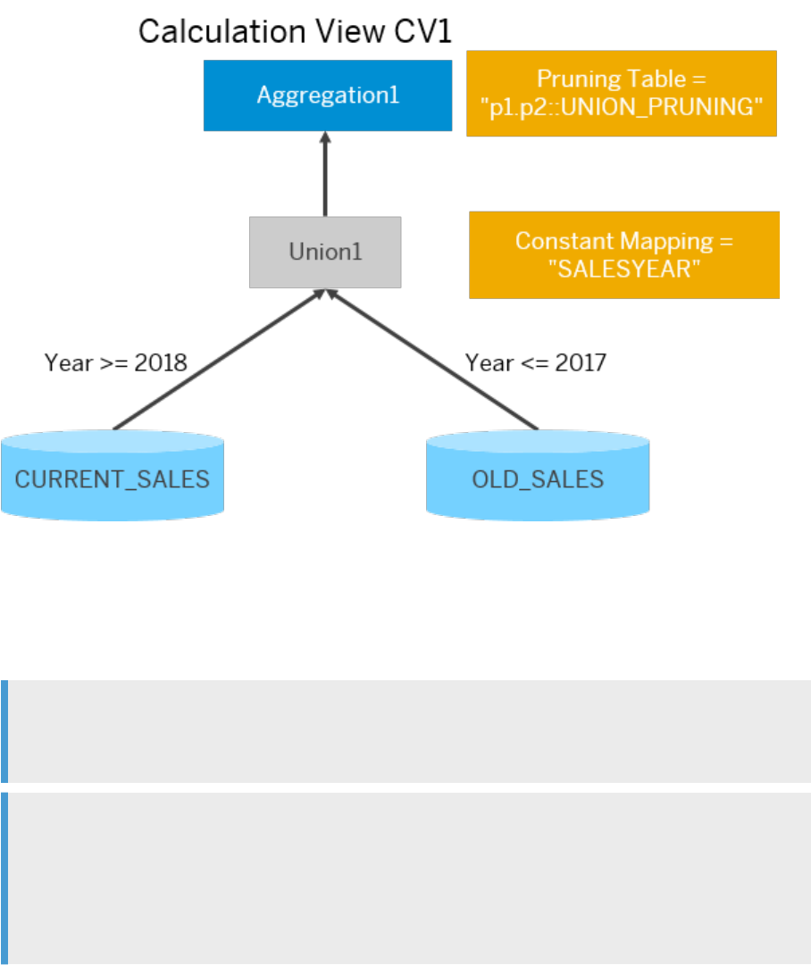
with the archived sales data (YEAR <= 2017). Both are provided as input to a union node in the calculation view,
as shown below:
In your scenario, you want to query the calculation view to get the results of CURRENT_SALES only. You
therefore want the query to be executed on the CURRENT_SALES data source only, and the operation on the
archived data source to be excluded (that is, pruned). To do so, you have the following options:
● You provide a pruning denition in a pruning conguration table.
● You create a constant that maps the data sources to specic constant values.
Note
In general, constant mapping improves performance more but is less exible than using a pruning
conguration table.
Note
If a union node is consumed by a rank node, query lters will, by default, not be pushed down to it when the
query is executed. This applies to lter expressions and variables used in a WHERE clause. However, to be
able to apply pruning, the union node needs the lters. In these cases, therefore, the combination of rank
node and union node with pruning only makes sense if the Allow Filter Push Down option has been activated
for the rank node.
Related Information
Pruning Conguration Table [page 222]
SAP HANA Performance Guide for Developers
Optimization Features in Calculation Views
P U B L I C 221
Example with a Pruning Conguration Table [page 222]
Example with a Constant Mapping [page 225]
Example Tables [page 227]
Push Down Filters in Rank Nodes [page 248]
SAP Note 2752070
7.5.1 Pruning Conguration Table
A pruning denition in a pruning conguration table has a specic format.
The format of a pruning conguration table is as follows:
Column Name
Description
CALC_SCENARIO Fully qualied name of the calculation view to which union node pruning
is to be applied. For example, p1.p2::CV_PRUNING, where p1.p2 is the
namespace and CV_PRUNING is the name of the calculation view.
INPUT Name of the data source in the union node of the calculation view.
COLUMN Target column name
OPTION Operator (=, <, >, <=, >=, BETWEEN)
LOW_VALUE Filter condition
HIGH_VALUE Filter condition
To assign a pruning conguration table to a calculation view, select the Semantics node and choose View
Properties
Advanced . Note that if you have not already created a pruning conguration table, you can both
create and build it from here.
7.5.2 Example with a Pruning Conguration Table
In this example, you use a pruning conguration table to specify the lter conditions for pruning the union
node. A matching lter is then applied in the WHERE clause of the query so that only one of the data sources is
processed.
Context
The calculation view is based on the example shown earlier. The Union node is used to combine the two data
sources Current_Sales and Old_Sales. In the procedure below, you query the calculation view to get the current
sales results only.
222
P U B L I C
SAP HANA Performance Guide for Developers
Optimization Features in Calculation Views
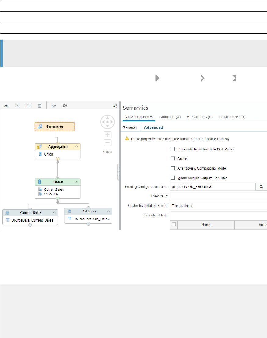
Procedure
1. Create a pruning denition in a pruning conguration table. For example:
Table: UNION_PRUNING
CALC_SCENARIO INPUT COLUMN OPTION LOW_VALUE HIGH_VALUE
1 p1.p2::CV_PRUNING OldSales YEAR <= 2017 NULL
2 p1.p2::CV_PRUNING CurrentSales YEAR >= 2018 NULL
Note
You can also create the table within step 3.
2. In the calculation view, select the Semantics node and choose View Properties Advanced .
3. In the Pruning Conguration Table eld, use the search to nd and add the pruning conguration table
created above, or choose + to create the table. For example:
The calculation view now contains the pruning conguration table with the two data sources CurrentSales
and OldSales.
4. Build the calculation view.
5. Execute a query on the calculation view with a lter condition that is the same as the condition dened in
the pruning conguration table. For example:
SELECT
"SALESORDER",
"PRODUCT",
"YEAR",
SUM("SALES") AS "SALES"
FROM "JOINCARDINALITYEXAMPLE_HDI_DB_1"."p1.p2::CV_PRUNING"
WHERE "YEAR" >= '2018'
GROUP BY "SALESORDER", "PRODUCT", "YEAR";
6. From the Run dropdown menu, choose Analyze SQL.
SAP HANA Performance Guide for Developers
Optimization Features in Calculation Views
P U B L I C 223
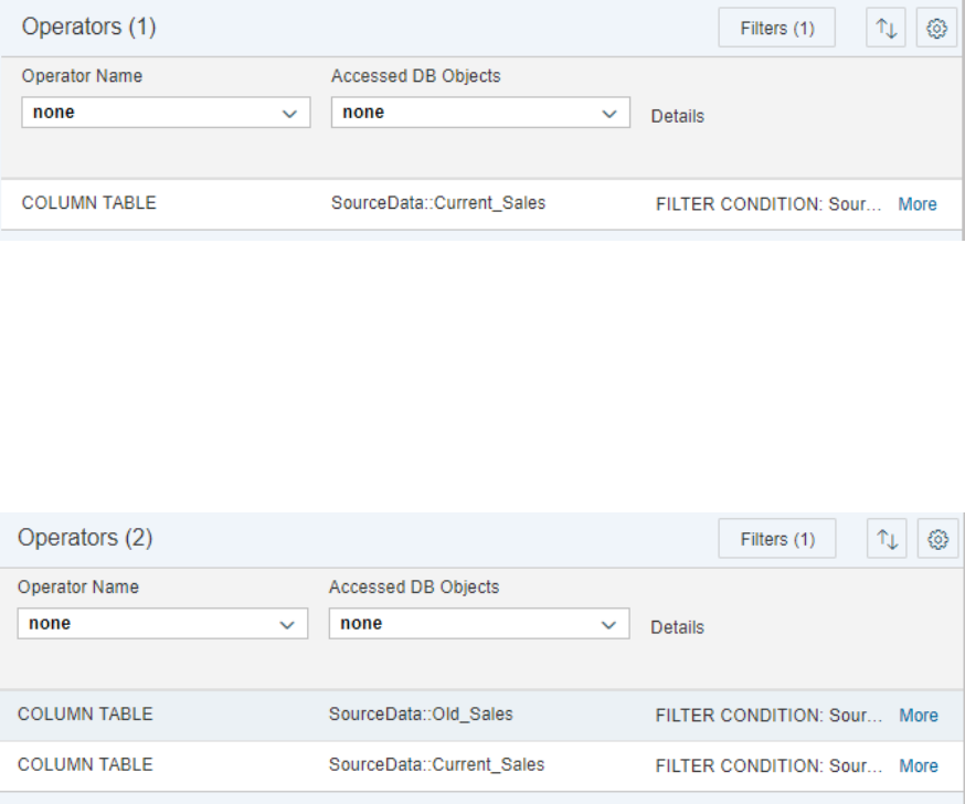
7. On the Operators tab, lter by the Column Table operator.
As can be seen, only the Current_Sales table is accessed. For example:
This conrms that the union node could be pruned because the lter condition matches the one in the
pruning conguration table.
8. Remove the pruning conguration table from the view properties of the calculation view and build it again.
9. Enter the same query as above and choose Analyze SQL from the Run dropdown menu.
10. On the Operators tab, lter by the Column Table operator.
As can be seen, the query is now invoking both the archived sales data and current sales data, although
only the current sales data is required. For example:
The presence of the Old_Sales table indicates that the union node was not pruned.
Results
As demonstrated therefore, union node pruning in calculation views allows the execution ow to be determined
dynamically based on the query. This allows resource consumption to be reduced and performance improved.
224
P U B L I C
SAP HANA Performance Guide for Developers
Optimization Features in Calculation Views
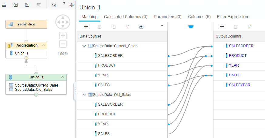
7.5.3 Example with a Constant Mapping
In this example, you use a constant to dene the criteria for pruning the union node and then apply it in the
WHERE clause of the query.
Context
The calculation view is based on the example shown earlier. The Union node is used to combine the two data
sources Current_Sales and Old_Sales. In the procedure below, you use the debug feature to visualize the
pruning.
Procedure
1. Create a calculation view with a Union node as follows:
2. Create a constant to dierentiate between the two dierent data sources:
a. On the Mapping tab of the Union node, choose + (Create Constant) in the Output Columns toolbar.
b. Enter the details required to dierentiate between the two data sources. For example:
SAP HANA Performance Guide for Developers
Optimization Features in Calculation Views
P U B L I C 225
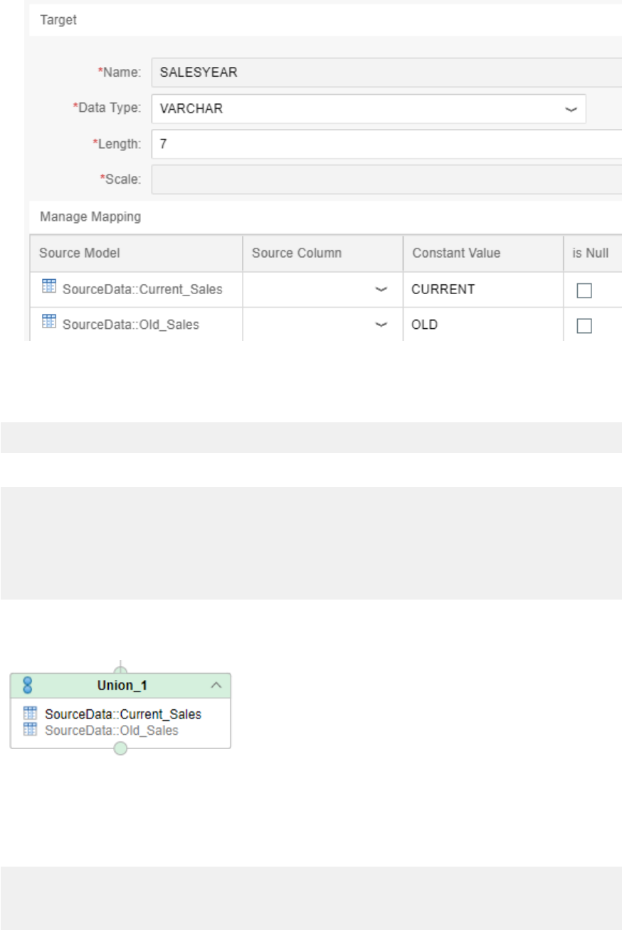
3. Save and build the calculation view.
4. To start debugging, select the Semantics node and then choose the Debug button.
5. On the Debug Query tab, add the following WHERE clause to the default debug query:
WHERE "SALESYEAR" = 'CURRENT'
For example:
SELECT "SALESORDER",
"PRODUCT",
"YEAR",
SUM("SALES") AS "SALES"
FROM "JOINCARDINALITYEXAMPLE_HDI_DB_1"."p1.p2::UNION_PRUNING"
WHERE "SALESYEAR" = 'CURRENT'
GROUP BY "SALESORDER", "PRODUCT", "YEAR", "SALESYEAR";
6. Click Execute to run the query.
The Old_Sales data source is now grayed out, indicating that is not being processed. For example:
The reason why it has been excluded is that the SALESYEAR lter does not match the constant value OLD
that you dened for it.
7. Rerun the debug query but replace CURRENT with OLD.
For example:
SELECT "SALESORDER",
"PRODUCT",
"YEAR",
SUM("SALES") AS "SALES"
226
P U B L I C
SAP HANA Performance Guide for Developers
Optimization Features in Calculation Views
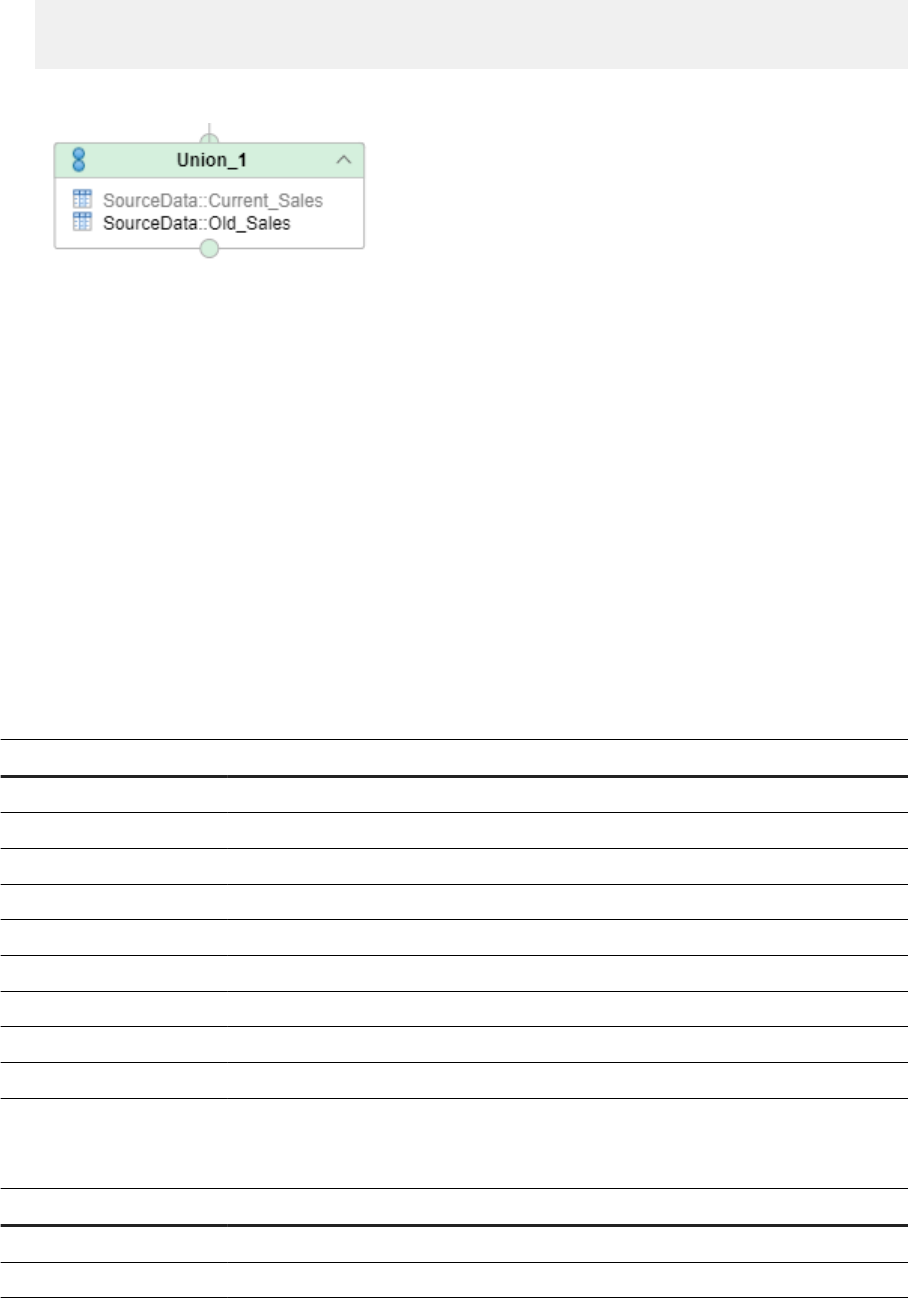
FROM "JOINCARDINALITYEXAMPLE_HDI_DB_1"."p1.p2::UNION_PRUNING"
WHERE "SALESYEAR" = 'OLD'
GROUP BY "SALESORDER", "PRODUCT", "YEAR", "SALESYEAR";
This time the Current_Sales data source is grayed out. For example:
Results
As shown above, when a constant is added to the union node of a calculation view, queries that apply a lter on
that constant will prune the applicable data sources in the Union node. This technique can be used to improve
the runtimes of complex models.
7.5.4 Example Tables
The following tables are used in the examples.
Current_Sales
SALESORDER PRODUCT YEAR SALES
006 PROD1 2018 450
006 PROD2 2018 330
006 PROD3 2018 510
007 PROD3 2018 1020
007 PROD1 2018 1350
007 PROD2 2018 990
008 PROD1 2018 450
008 PROD2 2018 330
009 PROD1 2018 900
009 PROD3 2018 1020
Old_Sales
SALESORDER PRODUCT YEAR SALES
001 PROD3 2016 510
001 PROD1 2016 450
SAP HANA Performance Guide for Developers
Optimization Features in Calculation Views
P U B L I C 227
Old_Sales
SALESORDER PRODUCT YEAR SALES
001 PROD2 2016 330
002 PROD1 2017 900
002 PROD3 2017 1020
002 PROD2 2017 660
003 PROD3 2017 510
004 PROD1 2017 450
004 PROD3 2017 510
005 PROD2 2017 330
7.6 Inuencing the Degree of Parallelization
SAP HANA uses an involved algorithm to determine the degree of parallelization with which queries are
executed. However, there might be situations where you want to inuence the degree of parallelization on top
of the general SAP HANA mechanism and control it explicitly for individual parts of your models based on
business considerations.
SAP HANA calculation views provide an option for doing this. But note that while this might be a helpful option
for individual highly time-critical models, it should not be used in an uncontrolled way because the overall
parallelization in SAP HANA might otherwise be negatively aected.
You can control parallel execution by modeling the number of logical threads to be used to execute specic
parts of the model. The term logical threads is used because parallelization is described from the perspective
of the model. Each logical thread might be further parallelized based on SAP HANA parallelization
optimizations. For example, an aggregation node can be parallelized into 6 logical threads based on the model
denition. Within each logical thread, additional parallelization might occur irrespective of the model settings.
A ag called Partition Local Execution indicates the start and stop nodes between which the degree of logical
parallelization is dened. The start ag needs to be set on a node that is based on a table. Typically, this is a
projection or an aggregation node. This node indicates the beginning of the parallelization. The end of
parallelization is denoted by a union node in which this ag is set again.
The degree of parallelization is dened at the node where the start ag is set.
Parallelization Based on Table Partitions
The degree of parallelization can be determined by the number of partitions in the table used as the data
source of the start node. Parallelization based on table partitions can be particularly helpful in scale-out
solutions where data needs to be transferred between dierent hosts. Imagine a table whose partitions are
distributed over several hosts. Without parallelization based on table partitioning, data from the individual
partitions would be sent over the network in order to be processed according to the model on one host. With
228
P U B L I C
SAP HANA Performance Guide for Developers
Optimization Features in Calculation Views

parallelization based on table partitioning, the logic that is modeled in the parallelization block would be
processed on the local host on which the table partitions are located. This local processing would not only
distribute the processing load but would probably also reduce the number of records that need to be sent over
the network. Therefore, it is a good idea to include an aggregation node at the end of your parallelization block
to reduce the amount of data before it is sent over the network.
Parallelization Based on Distinct Entries in a Column
Alternatively, the degree of parallelization can be determined by the number of distinct values in a column of
the table that serves as the data source of the start node.
Note
The Partition Local Execution ag gives you a high level of control over the degree of parallelization for
certain parts of your models based on your business logic and their relevance. Parallelization based on
table partitioning can be particularly helpful in scenarios in which tables are distributed across several
hosts. However, care must be taken when inuencing parallelization through modeling to avoid over-
parallelizing all models at the cost of other processes.
Related Information
Example: Create the Table [page 229]
Example: Create the Model [page 230]
Example: Apply Parallelization Based on Table Partitions [page 233]
Example: Apply Parallelization Based on Distinct Entries in a Column [page 236]
Verifying the Degree of Parallelization [page 238]
Constraints [page 241]
7.6.1 Example: Create the Table
The following table is used in the parallelization examples.
Procedure
Create the table partitionedTable.hdbtable with the following table denition:
COLUMN TABLE "tables::partitionedTable" ("SalesOrderId" NVARCHAR(10) NOT NULL
COMMENT 'Sales Order ID',
"CreatedBy" NVARCHAR(10) NOT NULL COMMENT 'Created By',
"CreatedAt" DATE CS_DAYDATE NOT NULL COMMENT 'Created At - Date and Time',
"ChangedBy" NVARCHAR(10) COMMENT 'Last Changed By',
SAP HANA Performance Guide for Developers
Optimization Features in Calculation Views
P U B L I C 229

"ChangedAt" DATE CS_DAYDATE COMMENT 'Last Changed At - Date and Time',
"NoteId" NVARCHAR(10) COMMENT 'SO Note Text ID',
"PartnerId" NVARCHAR(10) COMMENT 'Partner ID',
"Currency" NVARCHAR(5) NOT NULL COMMENT 'Currency Code',
"GrossAmount" DECIMAL(15,2) CS_FIXED DEFAULT 0 NOT NULL COMMENT 'Total
Gross Amount',
"NetAmount" DECIMAL(15,2) CS_FIXED DEFAULT 0 NOT NULL COMMENT 'Total Net
Amount',
"TaxAmount" DECIMAL(15,2) CS_FIXED DEFAULT 0 NOT NULL COMMENT 'Total Tax
Amount',
"LifecycleStatus" NVARCHAR(1) COMMENT 'SO Lifecycle Status',
"BillingStatus" NVARCHAR(1) COMMENT 'Billing Status',
"DeliveryStatus" NVARCHAR(1) COMMENT 'Delivery Status',
PRIMARY KEY ("SalesOrderId")) UNLOAD PRIORITY 5 AUTO MERGE PARTITION BY
HASH ("SalesOrderId") PARTITIONS 6
7.6.2 Example: Create the Model
The following model is used in the parallelization examples.
Procedure
1. Create the calculation view.
The calculation view consists of a projection node (startParallelization) that feeds into an
aggregation node (runInParallel), which in turn feeds into a union node (stopParallelization).
230
P U B L I C
SAP HANA Performance Guide for Developers
Optimization Features in Calculation Views
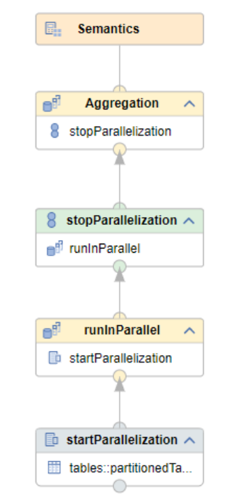
For example:
2. To trigger the aggregation in the aggregation node, do not map all columns to the output. For example:
SAP HANA Performance Guide for Developers
Optimization Features in Calculation Views
P U B L I C 231
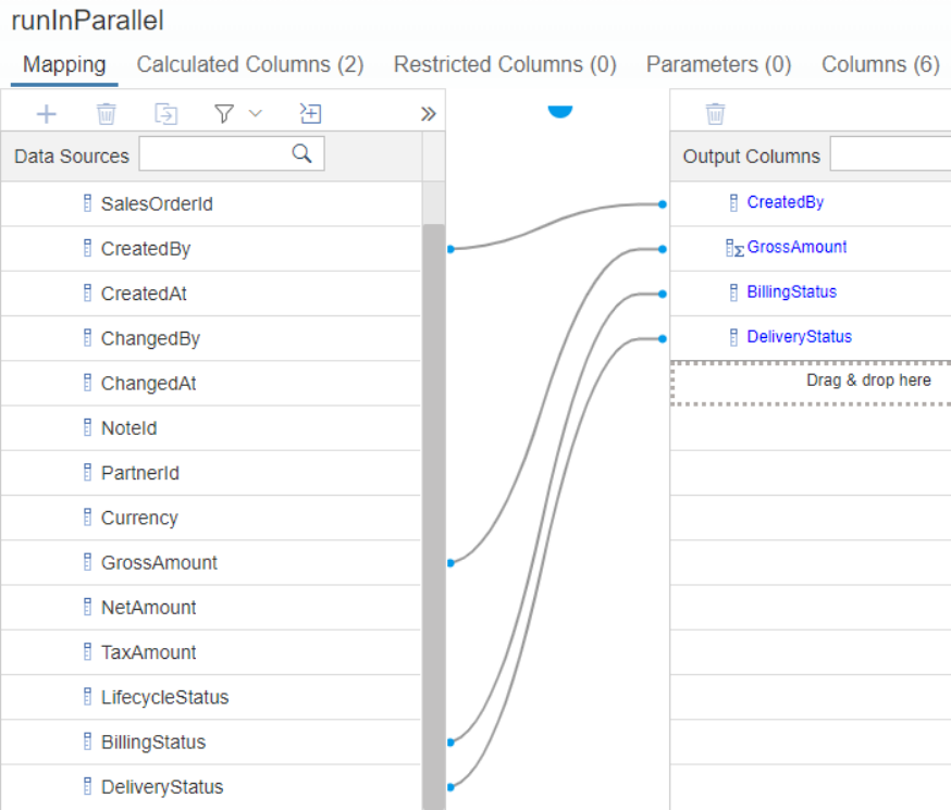
Aggregation is enforced because the output columns are a subset of the input columns.
3. Dene a calculated column in the aggregation node. For example:
232
P U B L I C
SAP HANA Performance Guide for Developers
Optimization Features in Calculation Views
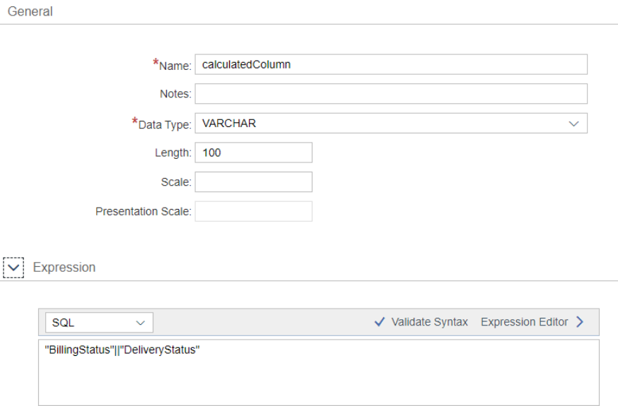
The calculated column in the aggregation node will be parallelized later.
7.6.3 Example: Apply Parallelization Based on Table
Partitions
This example shows how you can control parallelization in your model using table partitions.
Procedure
1. Dene the start node for parallelization:
a. Select the projection node startParallelization.
b. On the Mapping tab, select the data source.
c. Under Properties, select the Partition Local Execution option:
SAP HANA Performance Guide for Developers
Optimization Features in Calculation Views
P U B L I C 233
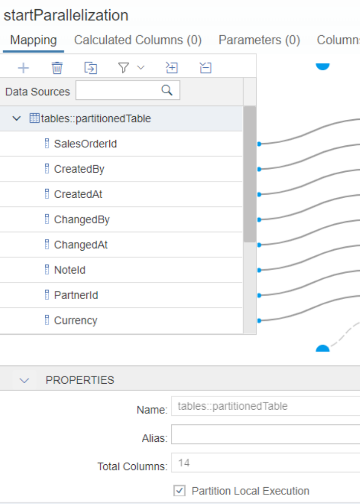
2. Dene the stop node for parallelization:
a. Select the union node stopParallelization.
b. On the Mapping tab, select the data source.
c. Under Properties, select the Partition Local Execution option:
234
P U B L I C
SAP HANA Performance Guide for Developers
Optimization Features in Calculation Views
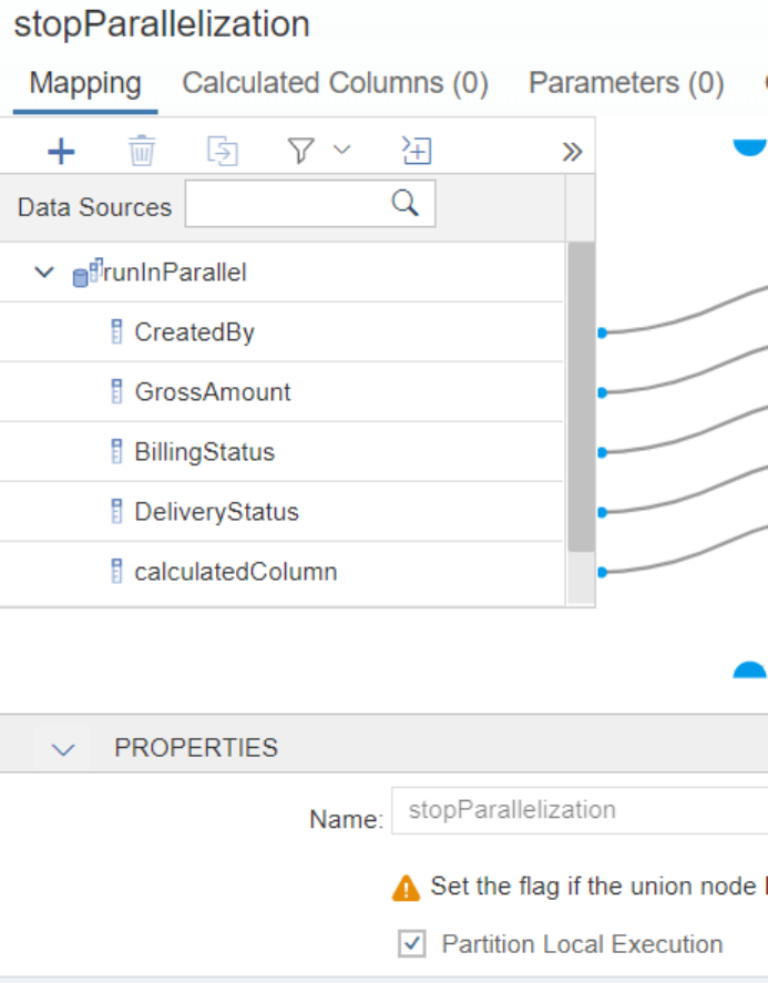
Results
Every node between the startParallelization and stopParallelization nodes will be executed in
parallel for each partition of the data source table of the startParallelization node. For the sake of
simplicity, only one node was inserted between the start and stop nodes of the parallelization block, but you
could have multiple nodes between the start and stop nodes.
SAP HANA Performance Guide for Developers
Optimization Features in Calculation Views
P U B L I C 235
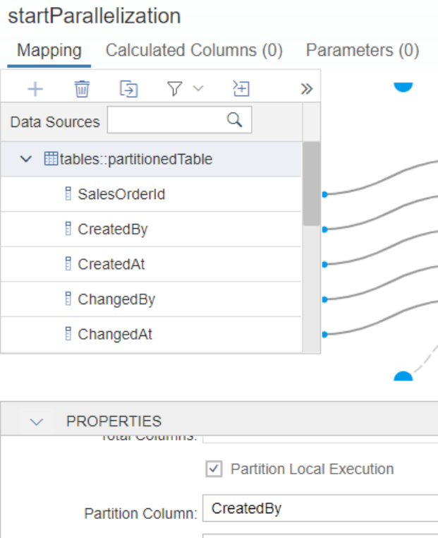
7.6.4 Example: Apply Parallelization Based on Distinct
Entries in a Column
This example shows how you can control parallelization in your model using distinct entries in a table column.
Procedure
1. Dene the start node for parallelization:
a. Select the projection node startParallelization.
b. On the Mapping tab, select the data source.
c. Under Properties, select the Partition Local Execution option.
d. Enter CreatedBy in the Partition Column eld:
2. Dene the stop node for parallelization:
a. Select the union node stopParallelization.
b. On the Mapping tab, select the data source.
236
P U B L I C
SAP HANA Performance Guide for Developers
Optimization Features in Calculation Views
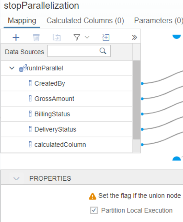
c. Under Properties, select the Partition Local Execution option:
Results
Every node between the startParallelization and stopParallelization nodes will be executed in
parallel for each distinct value in the CreatedBy column of the data source table of the
startParallelization node. For the sake of simplicity, only one node was inserted between the start and
stop nodes of the parallelization block, but you could have multiple nodes between the start and stop nodes.
SAP HANA Performance Guide for Developers
Optimization Features in Calculation Views
P U B L I C 237
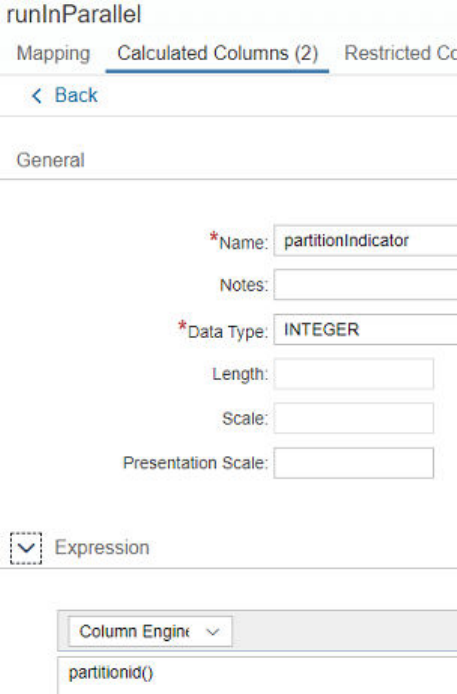
7.6.5 Verifying the Degree of Parallelization
You can verify the degree of parallelization at runtime by adding a calculated column that contains the logical
partition ID, or by using the SQL Analyzer, or by tracing query execution. All methods work both for
parallelization based on table partitions and parallelization based on distinct entries.
Adding a Calculated Column that Contains the Logical Partition ID
To see the ID of the logical thread that processed a certain record, you can add the column engine expression
partitionid() as a calculated column and display this column in the results.
For example, you can add a calculated column that evaluates the partition identier as shown below:
Assuming that parallelization is based on a table that consists of 6 partitions, you will see an integer between 1
and 6 for each record. The number corresponds to the logical thread that processed the record. This means
that records with the same partition ID were processed by the same thread.
238
P U B L I C
SAP HANA Performance Guide for Developers
Optimization Features in Calculation Views
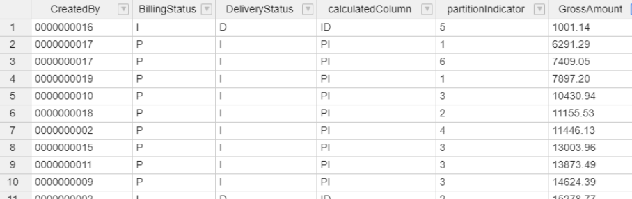
For example:
The calculated column partitionIndicator, which is lled by the column engine expression
partitionid(), indicates the logical thread that processed the record.
Using the SQL Analyzer
The SQL Analyzer can be used to check whether parallelization has been applied. To do so, you need to run the
SQL Analyzer for your statement and navigate to the nodes that should have been parallelized. For example, if
the parallelization is based on six partitions of a table, the nodes would be shown six times.
In the following example, the SQL Analyzer shows six parallel processing threads for the aggregation. The
aggregation node is grouped into ve identical nodes plus an additional aggregation node where the processing
is merged:
SAP HANA Performance Guide for Developers
Optimization Features in Calculation Views
P U B L I C 239
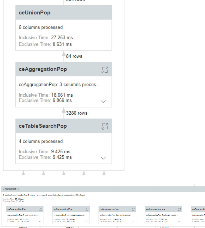
● The sixth node (aggregation):
● The ve nodes:
240
P U B L I C
SAP HANA Performance Guide for Developers
Optimization Features in Calculation Views
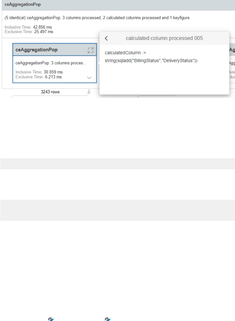
By drilling down into the aggregation ceAggregationPop, you can nd the calculated columns that were
parallelized. As the example below shows, the calculated column is evaluated in each parallel thread:
Tracing Query Execution
By tracing query execution, you can also check whether parallelization has been applied.
You can trace an individual query by adding the following, for example, to the query:
WITH PARAMETERS ('PLACEHOLDER' = ('$$CE_SUPPORT$$',"))
When you execute the query, a trace le with details about the calculation view execution will be created and
stored as an index server trace le with a name that ends in _cesupport.trc.
When you open the trace le, you should see something like the following:
"Partitioned execution rule: 6 partitions found for table
'LD0::EXAMPLEPARALLELIZATION_HDI_DB:tables::partitionedTable (t -1)'.
The partitioned execution branch will be cloned."
7.6.6 Constraints
The constraints that apply when using the parallelization setting are listed below:
● The start of parallelization can only be dened in the nodes with the table data source (the lowermost
nodes).
● Parallelization is not supported across views.
● Only one parallelization block is allowed per query.
● Multiple start parallelization nodes are allowed only if a parallelization column is dened.
Also note that setting the parallelization ag will block unfolding (for background information about unfolding,
see SAP Note 2291812 and SAP Note 2223597 ).
SAP HANA Performance Guide for Developers
Optimization Features in Calculation Views
P U B L I C 241
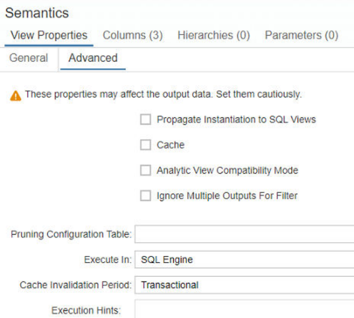
7.7 Using "Execute in SQL Engine" in Calculation Views
The Execute in SQL Engine option allows you to override the default execution behavior in calculation views.
When calculation views are included in queries, the query is rst optimized in the calculation engine. This has a
drawback when the query is included in a larger SQL query. This is because two dierent optimization
processes are then involved, one for the SQL query itself and one for the calculation view. This can lead to
ineciencies between the dierent optimization processes.
To avoid these ineciencies, a global optimization is applied automatically. This means that after certain
calculation engine-specic optimizations have been applied, the resulting plan is translated into an SQL
representation, referred to as a "QO" (query optimization), which allows the SQL optimizer to work on the
whole query. The translation into an SQL representation is called "unfolding". For more information about
unfolding, see SAP Notes 2618790 and 2223597, for example.
However, some calculation view features cannot be readily translated into an SQL optimization due to their
non-relational behavior. As a result, the unfolding process is blocked for the whole calculation view. In such
situations, you can direct the calculation engine to try to unfold parts of the view even though the view itself
cannot be fully unfolded. You can do this by setting the Execute in SQL Engine option. For example:
The most prominent features that block unfolding are queries that include non-SQL hierarchy views and
anonymization nodes.
The Execute in SQL Engine option improves the runtime in some queries, since recent optimizations have
focused on unfolded queries. Unfortunately, there is no general rule for determining when this option will lead
to performance improvements. Ideally, it will not be needed because the query will be unfolded anyway.
242
P U B L I C
SAP HANA Performance Guide for Developers
Optimization Features in Calculation Views
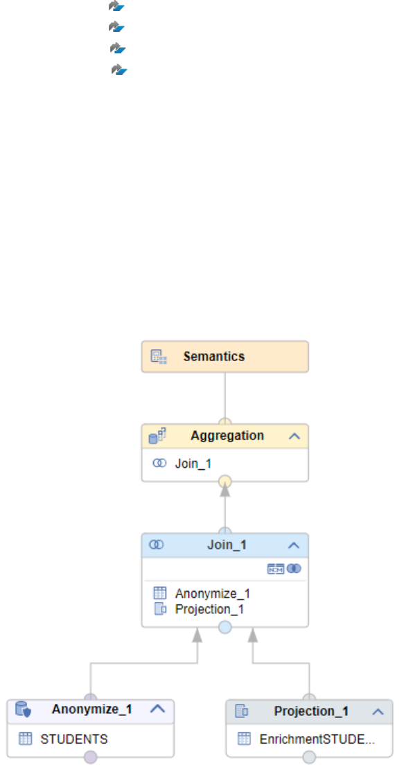
Nevertheless, there could be queries that cannot currently be unfolded. In these cases, setting the Execute in
SQL Engine option can sometimes help depending on the context in which the query is run.
Related Information
SAP Note 2618790
SAP Note 2223597
SAP Note 1857202
SAP Note 2441054
Impact of the "Execute in SQL Engine" Option [page 243]
Checking Whether a Query is Unfolded [page 246]
Inuencing Whether a Query is Unfolded [page 246]
7.7.1 Impact of the "Execute in SQL Engine" Option
The mechanism of the Execute in SQL Engine option is illustrated using a calculation view in which a feature
prevents unfolding. This feature is k-anonymity.
The following calculation view is used in this example. It includes an anonymization node as well as a join with a
table:
SAP HANA Performance Guide for Developers
Optimization Features in Calculation Views
P U B L I C 243
Due to the anonymization node, the calculation view cannot be fully unfolded. If Execute in SQL Engine is not
set, unfolding is blocked, and all optimization therefore occurs in the calculation engine. If you set the Execute
in SQL Engine option, all parts of the plan that can be translated into an SQL representation will be unfolded.
This is eective for the view on which the ag is set as well as its included views. As a result, unfolding is not
blocked for the entire view but only for parts of the plan.
In this example, an SQL translation of a join and data retrieval is created but the anonymization itself is not
unfolded. You can conrm that this is the case by analyzing the SQL plan:
The plan on the left shows the execution when the Execute in SQL Engine option is set. The plan on the right is
when the Execute in option is left empty. The ceQoPop operators on the left are the SQL representation of the
parts of the calculation engine plan that could be translated even though the calculation view as whole could
244 P U B L I C
SAP HANA Performance Guide for Developers
Optimization Features in Calculation Views
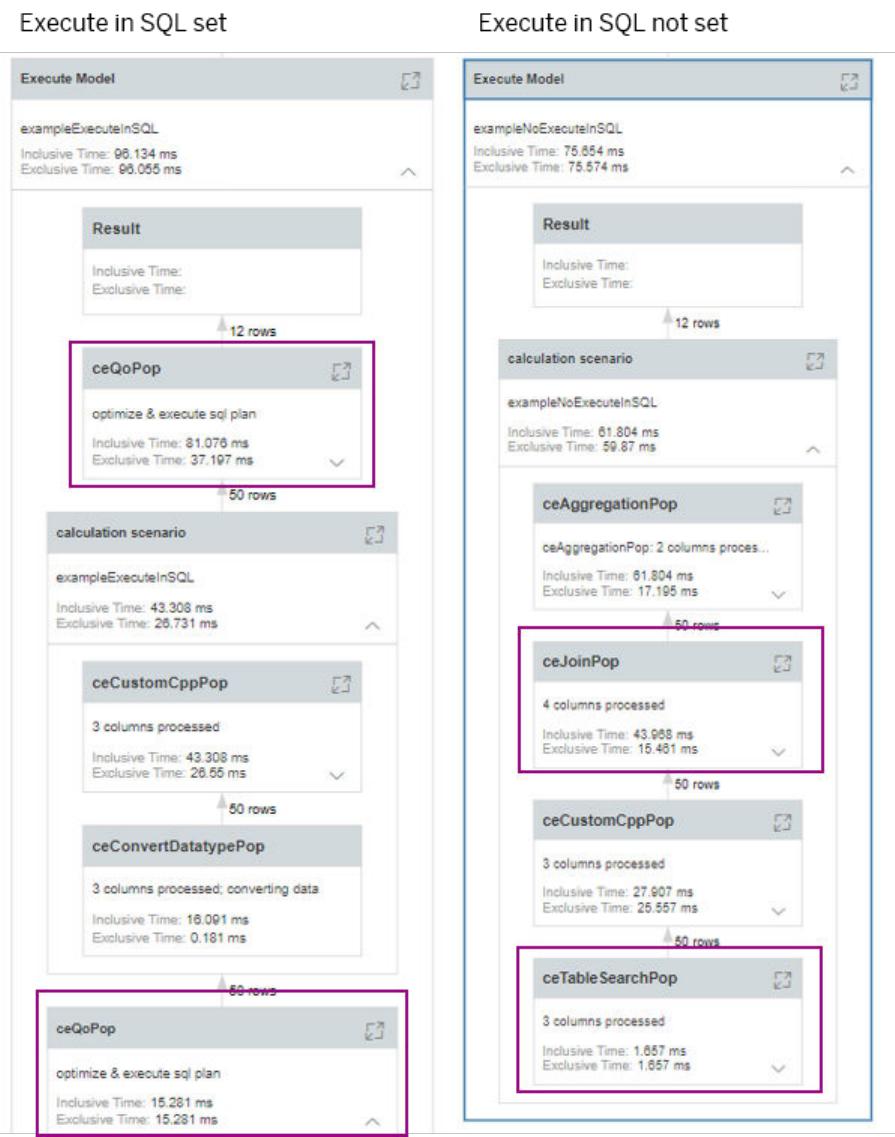
not be unfolded. In contrast, there are no ceQoPop operators on the right and optimization is done in the
calculation engine only:
On the left, the rst ceQoPop operator (bottom left) retrieves the data for the anonymization node and the
second
ceQoPop operator executes the join. On the right, the table is read with a calculation engine operator
SAP HANA Performance Guide for Developers
Optimization Features in Calculation Views
P U B L I C 245
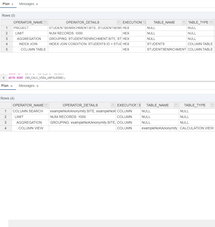
(bottom right) and the join is executed using calculation engine operators. This conrms that by setting the
Execute in SQL Engine option, you can enforce partial unfolding even if global unfolding of the view is blocked.
7.7.2 Checking Whether a Query is Unfolded
To check whether a query is unfolded, you can use the Explain Plan functionality. If all tables that are used in
the query appear in the plan, unfolding has taken place successfully.
The example below shows the Explain Plan of a query that is executed on the calculation view above. The k-
anonymity node has been replaced with a projection node. Unfolding therefore takes place, by default, and all
tables involved are shown in the plan:
Since the calculation view is unfolded by default, the hint NO_CALC_VIEW_UNFOLDING is used in the example
below to block unfolding:
A column view is now shown, but no tables can be seen at the lowest level.
7.7.3 Inuencing Whether a Query is Unfolded
Unfolding is applied by default and you should avoid blocking it. Because the long-term goal is to unfold all
queries, future optimizations are highly focused on unfolded queries.
Several options are available for blocking unfolding (see SAP Note 2441054):
● Attach a hint to an individual statement: WITH HINT (NO_CALC_VIEW_UNFOLDING)
● Pin a hint to every execution of a statement (see SAP Note 2400006):
ALTER SYSTEM ADD STATEMENT HINT (NO_CALC_VIEW_UNFOLDING) FOR <sql_statement>
246
P U B L I C
SAP HANA Performance Guide for Developers
Optimization Features in Calculation Views
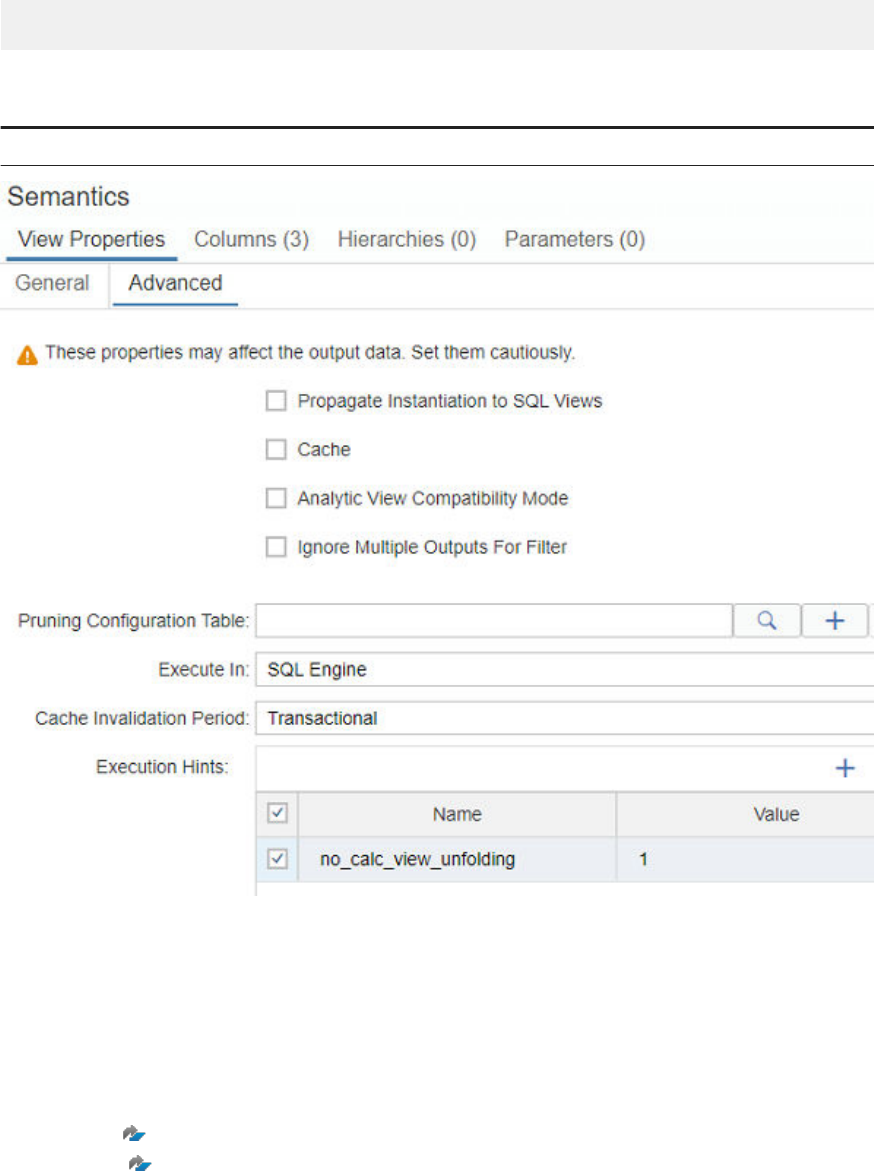
ALTER SYSTEM PIN SQL PLAN CACHE ENTRY <plan_id> WITH HINT
(NO_CALC_VIEW_UNFOLDING)
● Add the hint to a specic view using an execution hint in a calculation view:
Name Value
no_calc_view_unfolding 1
● Block unfolding globally by setting the conguration parameter
[calcengine]no_calc_view_unfolding to 1 in the indexserver.ini le.
Related Information
SAP Note 2441054
SAP Note 2400006
SAP HANA Performance Guide for Developers
Optimization Features in Calculation Views
P U B L I C 247

7.8 Push Down Filters in Rank Nodes
Filters used in a query are, by default, not pushed down by rank nodes. This applies to lter expressions and
variables used in a WHERE clause. In these cases, a rank node accesses all the data of the nodes below it. You
can override this behavior by setting the Allow Filter Push Down option.
Context
Set the Allow Filter Push Down option only if it is semantically correct for the particular use case.
Procedure
1. In the calculation view, select the rank node.
2. Choose the Mapping tab.
3. In the Properties section, select the Allow Filter Push Down option.
4. Save and build the calculation view.
Results
When the query is executed, the lter will be pushed down to the nodes below the rank node.
7.9 Condensed Performance Suggestions
The following table summarizes the main performance recommendations.
Performance Suggestion
Description
Join cardinality and key elds It is highly recommended to set a join cardinality because this makes the calcula
tion view easier to optimize.
Optimized join columns It is highly recommended to set the Optimize Join Columns option where appro
priate because it allows unnecessary columns to be pruned.
248 P U B L I C
SAP HANA Performance Guide for Developers
Optimization Features in Calculation Views
Performance Suggestion Description
Join columns and partitioning criteria in
scale-out scenarios
It is recommended to use matching partitions for tables that are joined.
The join columns should be used as the keys for partitioning tables. If the join col
umns are used for partitioning on both sides, the rst-level partition criteria must
be identical on both sides (particularly for round robin and hash partitioning).
This allows ecient parallel processing.
Join cardinality and referential integrity
It is recommended to provide as much information as possible about the calcula
tion model to support optimization.
When providing join cardinality information, check whether you can also provide
information about referential integrity.
Calculated attributes in join conditions
Calculated attributes should be avoided in join conditions because they might
prevent certain internal optimizations.
Calculated attributes in lter expres
sions
Calculated attributes should be avoided in lter expressions because they can
prevent certain internal optimizations related to lter pushdown.
Measures in join conditions Measures should not be used in join conditions because of potentially high car
dinalities that lead to longer runtimes.
Measures in lter expressions Measures should be avoided in lter expressions because they might prevent in
ternal optimizations.
Data type conversion in lters Data type conversion should be avoided in lters.
Ideally, it should not be necessary to convert data types. However, because a lter
must be dened with the correct format, it might be necessary to convert the
data types involved, for example, for comparison purposes. In these cases, it is
better to cast individual values from one data type to another within the lter ex
pression, rather than casting an entire column. For example, if column1 is com
pared to value1, it is preferable to convert value1 rather than column1.
= Recommended, = Problematic
SAP HANA Performance Guide for Developers
Optimization Features in Calculation Views
P U B L I C 249

7.10 Avoid Long Build Times for Calculation Views
When a calculation view takes a long time to build, it might be because it has many dependent hierarchy views.
Context
When you build a calculation view, all views based on the calculation view also need to be built. This can lead to
very long build times if there are many dependent views.
In general, you should try to reduce the number of views that are based on the calculation view you want to
build. You should also make sure that all views placed on top of the calculation view are valid views.
If the long build time is caused by the creation of technical hierarchies dened on the calculation view, it is
recommended that you check whether you can switch the data category of the calculation view to SQL
Access Only. This setting prevents technical hierarchies from being created.
The procedures below describe how to check whether long build times are caused by technical hierarchies and
how to set the data category of a calculation view to SQL Access Only.
Check Whether Long Build Times are Caused by Technical
Hierarchies
The diserver trace les provide information that can be used to analyze issues related to calculation view
build times.
Procedure
1. Set the trace level of the hana_di component of the diserver service to at least level INFO (the highest
trace level is DEBUG). You can do this from the SAP HANA cockpit or the SQL console:
Option
Description
SAP HANA cockpit 1. Click the Browse Database Objects tile. The SAP
HANA database explorer opens.
2. Select your database and from the context menu
choose
Trace Conguration.
3. In the Database Trace tile, click Edit. The Database
Trace Conguration dialog box opens.
4. Under DISERVER, set the trace level of hana_di to
INFO or higher.
5. Choose OK to save your settings.
250 P U B L I C
SAP HANA Performance Guide for Developers
Optimization Features in Calculation Views

Option Description
SQL ALTER SYSTEM ALTER CONFIGURATION
('diserver.ini', 'SYSTEM') SET
('trace', 'hana_di') = 'INFO';
2. Build the calculation view.
3. Open the current diserver trace le.
You can access the trace le from the SAP HANA cockpit or directly on operating system level:
Option
Description
SAP HANA cockpit 1. In the Alerting and Diagnostics tile, choose View trace
and diagnostic les. The SAP HANA database ex
plorer opens.
2. In the directory structure under Datatabase
Diagnostic Files, expand the diserver folder. The dis
erver trace les are named as follows:
diserver_<host>.<port>.<counter>.trc
Operating system level
/usr/sap/<sid>/HDB<inst>/<host>/trace/
diserver_<host>.<port>.<counter>.trc
4. In the diserver trace le, check whether both of the following conditions apply:
○ You can nd a lot of entries that are related to views (for example, CREATE VIEW, DROP VIEW). These
entries have the following pattern:<view_name>/<column_name>/hier/<column_name>
○ These statements take up a signicant amount of the overall build time.
Avoid Creating Technical Hierarchies (Optional)
Depending on the data category assigned to a calculation view, technical hierarchies are created for each
column of the view. Technical hierarchies are required for MDX queries.
Context
Calculation views are classied by one of the following data categories: CUBE, DIMENSION, or SQL ACCESS
ONLY. In the case of SQL ACCESS ONLY, technical hierarchies are not created. If your front-end tool does not
rely on technical hierarchies, you can avoid creating them by assigning this data category to the calculation
view. You can assign the data category either when you create the calculation view or later.
Procedure
● To create a calculation view with the SQL ACCESS ONLY data category, do the following:
a. In the New Calculation View dialog box, enter SQL ACCESS ONLY in the Data Category eld.
SAP HANA Performance Guide for Developers
Optimization Features in Calculation Views
P U B L I C 251

● To switch the data category of a calculation view that has been created as a CUBE or DIMENSION, proceed
as follows:
a. Double-click the Semantics node.
b. On the View Properties tab, enter SQL ACCESS ONLY in the Data Category eld.
c. Save the calculation view.
Note
If you change the data category from CUBE or DIMENSION to SQL ACCESS ONLY and the view is
directly accessed by a front-end tool, verify that the front-end tool can still report on the respective
view. Also, do not change the data category to SQL ACCESS ONLY if you have explicitly modeled
hierarchies in the Semantics node.
252 P U B L I C
SAP HANA Performance Guide for Developers
Optimization Features in Calculation Views

Important Disclaimers and Legal Information
Hyperlinks
Some links are classied by an icon and/or a mouseover text. These links provide additional information.
About the icons:
● Links with the icon : You are entering a Web site that is not hosted by SAP. By using such links, you agree (unless expressly stated otherwise in your
agreements with SAP) to this:
● The content of the linked-to site is not SAP documentation. You may not infer any product claims against SAP based on this information.
● SAP does not agree or disagree with the content on the linked-to site, nor does SAP warrant the availability and correctness. SAP shall not be liable for any
damages caused by the use of such content unless damages have been caused by SAP's gross negligence or willful misconduct.
● Links with the icon : You are leaving the documentation for that particular SAP product or service and are entering a SAP-hosted Web site. By using such
links, you agree that (unless expressly stated otherwise in your agreements with SAP) you may not infer any product claims against SAP based on this
information.
Beta and Other Experimental Features
Experimental features are not part of the ocially delivered scope that SAP guarantees for future releases. This means that experimental features may be changed by
SAP at any time for any reason without notice. Experimental features are not for productive use. You may not demonstrate, test, examine, evaluate or otherwise use
the experimental features in a live operating environment or with data that has not been suciently backed up.
The purpose of experimental features is to get feedback early on, allowing customers and partners to inuence the future product accordingly. By providing your
feedback (e.g. in the SAP Community), you accept that intellectual property rights of the contributions or derivative works shall remain the exclusive property of SAP.
Example Code
Any software coding and/or code snippets are examples. They are not for productive use. The example code is only intended to better explain and visualize the syntax
and phrasing rules. SAP does not warrant the correctness and completeness of the example code. SAP shall not be liable for errors or damages caused by the use of
example code unless damages have been caused by SAP's gross negligence or willful misconduct.
Gender-Related Language
We try not to use gender-specic word forms and formulations. As appropriate for context and readability, SAP may use masculine word forms to refer to all genders.
254
P U B L I C
SAP HANA Performance Guide for Developers
Important Disclaimers and Legal Information
SAP HANA Performance Guide for Developers
Important Disclaimers and Legal Information
P U B L I C 255

www.sap.com/contactsap
© 2019 SAP SE or an SAP aliate company. All rights reserved.
No part of this publication may be reproduced or transmitted in any form
or for any purpose without the express permission of SAP SE or an SAP
aliate company. The information contained herein may be changed
without prior notice.
Some software products marketed by SAP SE and its distributors
contain proprietary software components of other software vendors.
National product specications may vary.
These materials are provided by SAP SE or an SAP aliate company for
informational purposes only, without representation or warranty of any
kind, and SAP or its aliated companies shall not be liable for errors or
omissions with respect to the materials. The only warranties for SAP or
SAP aliate company products and services are those that are set forth
in the express warranty statements accompanying such products and
services, if any. Nothing herein should be construed as constituting an
additional warranty.
SAP and other SAP products and services mentioned herein as well as
their respective logos are trademarks or registered trademarks of SAP
SE (or an SAP aliate company) in Germany and other countries. All
other product and service names mentioned are the trademarks of their
respective companies.
Please see https://www.sap.com/about/legal/trademark.html for
additional trademark information and notices.
THE BEST RUN
